Difference between revisions of "Nonlinear Shallow Water Waves"
| (47 intermediate revisions by 3 users not shown) | |||
| Line 1: | Line 1: | ||
| + | {{nonlinear waves course | ||
| + | | chapter title = Nonlinear Shallow Water Waves | ||
| + | | next chapter = [[Introduction to KdV]] | ||
| + | | previous chapter = [[Traffic Waves]] | ||
| + | }} | ||
| + | |||
{{complete pages}} | {{complete pages}} | ||
| Line 8: | Line 14: | ||
This allows us to assume [[:Category:Shallow Depth|Shallow Depth]]. We assume that the problem has not variation | This allows us to assume [[:Category:Shallow Depth|Shallow Depth]]. We assume that the problem has not variation | ||
in either the <math>y</math> or <math>z</math> direction. The fluid is governed by two parameters, | in either the <math>y</math> or <math>z</math> direction. The fluid is governed by two parameters, | ||
| − | <math>u</math> and <math>h</math> the water depth ( | + | <math>u(x,t)</math>, the velocity of the water, and <math>h(x,t)</math> the water depth (note that this is not the still water depth since the problem |
is nonlinear). | is nonlinear). | ||
| Line 19: | Line 25: | ||
<center> | <center> | ||
<math> | <math> | ||
| − | \partial_t \int_x^{x + \Delta x} \rho h(s,t) | + | \partial_t \int_x^{x + \Delta x} \rho h(s,t) \mathrm{d}s = \rho h(x,t)u(x,t) - \rho h(x+\Delta x,t)u(x+\Delta x,t) |
</math> | </math> | ||
</center> | </center> | ||
| Line 33: | Line 39: | ||
<center> | <center> | ||
<math> | <math> | ||
| − | \partial_t \int_{x}^{x + \Delta x} \rho h u | + | \partial_t \int_{x}^{x + \Delta x} \rho h u \mathrm{d}x |
= \left. \rho u^2 h \right|_{x}^{x + \Delta x} | = \left. \rho u^2 h \right|_{x}^{x + \Delta x} | ||
| − | + \int_0^{h(x)} P( | + | + \int_0^{h(x)} P(x,z,t) \mathrm{d}z - |
| − | \int_0^{h(x + \Delta)} P( | + | \int_0^{h(x + \Delta x)} P(x+\Delta x,z,t) \mathrm{d}z |
</math> | </math> | ||
</center> | </center> | ||
| − | where the pressure <math>P</math> is given by | + | where <math>\rho \,</math> denotes density, and the pressure <math>P \,</math> is given by |
<center> | <center> | ||
<math> | <math> | ||
| Line 48: | Line 54: | ||
<center> | <center> | ||
<math> | <math> | ||
| − | \partial_t \int_{x}^{x + \Delta x} \rho h u | + | \partial_t \int_{x}^{x + \Delta x} \rho h u \mathrm{d}x |
| − | = \left. \rho u^2 h \right|_{x}^{x + \Delta x} | + | = -\left. \rho u^2 h \right|_{x}^{x + \Delta x} |
+ \frac{1}{2}\rho g {h(x)}^2 - | + \frac{1}{2}\rho g {h(x)}^2 - | ||
\frac{1}{2}\rho g {h(x + \Delta x)}^2 | \frac{1}{2}\rho g {h(x + \Delta x)}^2 | ||
| Line 58: | Line 64: | ||
<math> | <math> | ||
\partial_t \left( h u \right) | \partial_t \left( h u \right) | ||
| − | + | + \partial_x \left(u^2 h + \frac{1}{2} gh^2\right) =0 | |
</math> | </math> | ||
</center> | </center> | ||
| Line 128: | Line 134: | ||
<center> | <center> | ||
<math> | <math> | ||
| − | \frac{d X_+}{d t} = u + c = u + \sqrt{gh} | + | \frac{\mathrm{d} X_+}{\mathrm{d} t} = u + c = u + \sqrt{gh} |
</math> | </math> | ||
</center> | </center> | ||
| Line 141: | Line 147: | ||
<center> | <center> | ||
<math> | <math> | ||
| − | \frac{d X_-}{d t} = u - c = u - \sqrt{gh} | + | \frac{\mathrm{d} X_-}{\mathrm{d} t} = u - c = u - \sqrt{gh} |
</math> | </math> | ||
</center> | </center> | ||
| Line 163: | Line 169: | ||
[http://en.wikipedia.org/wiki/Hydraulic_jump hydraulic jump] | [http://en.wikipedia.org/wiki/Hydraulic_jump hydraulic jump] | ||
when it occurs on the surface of the water. | when it occurs on the surface of the water. | ||
| − | |||
| − | |||
=== The dam break problem === | === The dam break problem === | ||
| Line 199: | Line 203: | ||
<center> | <center> | ||
<math> | <math> | ||
| − | \frac{d X_\pm}{d t} = u \pm \sqrt{gh} = \pm c_0 | + | \frac{\mathrm{d} X_\pm}{\mathrm{d} t} = u \pm \sqrt{gh} = \pm c_0 |
</math> | </math> | ||
</center> | </center> | ||
| Line 211: | Line 215: | ||
<center> | <center> | ||
<math> | <math> | ||
| − | \frac{d X_-}{d t} = u - \sqrt{gh} | + | \frac{\mathrm{d} X_-}{\mathrm{d} t} = u - \sqrt{gh} |
</math> | </math> | ||
</center> | </center> | ||
| Line 256: | Line 260: | ||
the <math>C_+</math> characteristic only exist in the region <math>\big\{x < 2c_0 t \big\}</math>, | the <math>C_+</math> characteristic only exist in the region <math>\big\{x < 2c_0 t \big\}</math>, | ||
We will verify this by explicitly calculating them. | We will verify this by explicitly calculating them. | ||
| − | |||
| − | |||
| − | |||
| − | |||
| − | |||
It remains to determine the <math>C_+</math> characteristic, which originated in <math>\big\{x < 0 \big\}</math>, | It remains to determine the <math>C_+</math> characteristic, which originated in <math>\big\{x < 0 \big\}</math>, | ||
| Line 271: | Line 270: | ||
</math> | </math> | ||
</center> | </center> | ||
| − | When <math>t = \frac{x_0}{2c_0},\;\;\ | + | When <math>t = \frac{x_0}{2c_0},\;\;\ X_{+} (t) = -c_0 t</math> so that for |
<center> | <center> | ||
<math> | <math> | ||
| − | t > \frac{x_0}{2c_0},\ | + | t > \frac{x_0}{2c_0}, \quad \frac{\mathrm{d} X_{+} (t)}{\mathrm{d} t} = u + \sqrt{gh} |
</math> | </math> | ||
</center> | </center> | ||
| Line 280: | Line 279: | ||
<center> | <center> | ||
<math> | <math> | ||
| − | \frac{ | + | \frac{\mathrm{d}X_{+} (t)}{\mathrm{d} t} = \frac{4}{3}c_0 + \frac{X_{+} (t)}{3t} |
</math> | </math> | ||
</center> | </center> | ||
| Line 297: | Line 296: | ||
X_+ (t) = | X_+ (t) = | ||
\begin{cases} | \begin{cases} | ||
| − | 2c_0 t - 3\left(\frac{x_0}{2}\right)^{2/3}(c_0 t)^{1/3},\quad t> x_0/2\ | + | 2c_0 t - 3\left(\frac{x_0}{2}\right)^{2/3}(c_0 t)^{1/3},\quad t> x_0/2 c_0\ |
| − | -x_0 + | + | -x_0 + c_0 t, \quad 0\ < t < x_0/2 c_0 |
\end{cases} | \end{cases} | ||
</math> | </math> | ||
</center> | </center> | ||
| + | |||
| + | {| class="wikitable" | ||
| + | |- | ||
| + | ! Characteristics | ||
| + | ! Surface elevation | ||
| + | |- | ||
| + | | [[Image:Characteristics_dam_break.jpg|thumb|right|500px|Characteristics for the dam | ||
| + | break problem, blue for <math>C_{+}</math> and red for <math>C_{-}</math>. The solid red lines | ||
| + | show the curves <math>x=-c_0 t</math> and <math>x=2c_0 t</math> (note we have assumed | ||
| + | here that <math>c_0 =1</math>]] | ||
| + | | [[Image:Dambreak.gif|thumb|right|500px|Evolution of the fluid surface <math>h(x,t)</math> for the Dam Break problem]] | ||
| + | |} | ||
| + | |||
| + | == Shocks == | ||
| + | |||
| + | For a unique solution two exist there must be a single <math>C_+</math> and <math>C_-</math> | ||
| + | characteristic through each point. When two characteristics of the same kind meet we | ||
| + | have a shock forming. | ||
=== Accelerating Piston === | === Accelerating Piston === | ||
| Line 333: | Line 350: | ||
<center> | <center> | ||
<math> | <math> | ||
| − | u+2c = a t_0 + 2c_{\ | + | u+2c = a t_0 + 2c_{\text{plate}} \, |
</math> | </math> | ||
</center> | </center> | ||
where <math> a t_0</math> is the velocity of the piston at time <math>t=t_0</math> | where <math> a t_0</math> is the velocity of the piston at time <math>t=t_0</math> | ||
| − | and <math>c_{\ | + | and <math>c_{\text{plate}}</math> is the speed (related to height) at the plate. |
We know that <math> R_- = u - 2 c =-2c_0</math> through out the fluid, so that if | We know that <math> R_- = u - 2 c =-2c_0</math> through out the fluid, so that if | ||
| − | we solve this at the plate (where <math>u=at_0</math> and <math>c=c_{\ | + | we solve this at the plate (where <math>u=at_0</math> and <math>c=c_{\text{plate}}</math>) |
| − | then we get <math>c_{\ | + | then we get |
| + | <center><math> | ||
| + | c_{\text{plate}} = at_0/2 + c_0\, | ||
| + | </math></center> | ||
| − | + | On the <math>C_+</math> characteristics <math>u</math> and <math>c</math> | |
are constant and therefore | are constant and therefore | ||
<center> | <center> | ||
<math> | <math> | ||
| − | \frac{ | + | \frac{\mathrm{d}X_+}{\mathrm{d}t} = u+c = at_0 + \left( \frac{1}{2}at_0 + c_0 \right) |
</math> | </math> | ||
</center> | </center> | ||
| Line 355: | Line 375: | ||
</math> | </math> | ||
</center> | </center> | ||
| − | using the condition <math>X_+(t_0) = \frac{1}{2} a t_0^2</math> (the initial value which | + | using the condition <math>X_+(t_0,t_0) = \frac{1}{2} a t_0^2</math> (the initial value which |
comes from the position of the piston at <math>t=t_0</math>). | comes from the position of the piston at <math>t=t_0</math>). | ||
The slope of these lines increases and eventually meet to form a shock. | The slope of these lines increases and eventually meet to form a shock. | ||
| Line 362: | Line 382: | ||
<center> | <center> | ||
<math> | <math> | ||
| − | X_+(t,t_0 + \Delta t) = X_+(t,t_0) + \Delta t \frac{\partial X_+}{\partial t_0} (t,t_0) | + | X_+(t,t_0 + \Delta t) = X_+(t,t_0) + \Delta t \frac{\partial X_+}{\partial t_0} (t,t_0) = X_+(t,t_0) |
</math> | </math> | ||
</center> | </center> | ||
| Line 383: | Line 403: | ||
characteristics. | characteristics. | ||
| − | |||
| − | + | {| class="wikitable" | |
| − | + | |- | |
| − | + | ! Characteristics | |
| + | ! Surface elevation | ||
| + | |- | ||
| + | | [[Image:Accelerating_piston.jpg|thumb|right|500px| <math>C_{+}</math> characteristics for the | ||
| + | accelerating piston, red undisturbed, blue from the piston and the green line shows the transition.]] | ||
| + | | [[Image:Accelerating_piston2.gif|thumb|right|500px|Evolution of the fluid surface <math>h(x,t)</math> for the | ||
| + | accelerating piston.]] | ||
| + | |} | ||
=== Piston Moving with Constant Velocity === | === Piston Moving with Constant Velocity === | ||
| − | + | This example is also known as the Moving Wall Problem, and is connected to Shallow Water Bores. | |
| − | + | ||
| − | fluid | + | We consider the case of a piston, with positive constant velocity <math>V</math> (which is initially at <math>x=0</math>), advancing into a semi-infinite expanse of |
| + | fluid that is initially at rest with depth <math>h_0</math>. | ||
| + | |||
The <math>C_+</math> characteristics which originate in the fluid | The <math>C_+</math> characteristics which originate in the fluid | ||
at <math>t=0</math> have slope | at <math>t=0</math> have slope | ||
<center> | <center> | ||
| − | <math>\frac{d X_+}{ | + | <math>\frac{\mathrm{d} X_+}{\mathrm{d}t} = \sqrt{gh_0}</math> |
</center> | </center> | ||
and the <math>C_+</math> characteristic which originate at the piston at | and the <math>C_+</math> characteristic which originate at the piston at | ||
<math>t=0</math> must satisfy | <math>t=0</math> must satisfy | ||
<center> | <center> | ||
| − | <math>\frac{d X_+}{ | + | <math>\frac{\mathrm{d} X_+}{\mathrm{d}t} = \sqrt{gh_0} + \frac{3}{2} V </math> |
</center> | </center> | ||
so that these two characteristics will intersect at <math>t=0</math>. | so that these two characteristics will intersect at <math>t=0</math>. | ||
| Line 414: | Line 442: | ||
<center> | <center> | ||
<math> | <math> | ||
| − | \partial_t \int_{x_1}^{x_2} \rho h | + | \partial_t \int_{x_1}^{x_2} \rho h \mathrm{d}x |
| − | + \left. \rho u h \right|_{ | + | + \left. \rho u h \right|_{x_2}^{x_1} =0 |
</math> | </math> | ||
</center> | </center> | ||
If the shock is located at <math>s(t)</math> | If the shock is located at <math>s(t)</math> | ||
which we assume is located between <math>x_1</math> | which we assume is located between <math>x_1</math> | ||
| − | and <math>x_2</math>, then | + | and <math>x_2</math>, then |
<center> | <center> | ||
<math> | <math> | ||
| − | \partial_t \int_{x_1}^{x_2} \ | + | \partial_t \int_{x_1}^{x_2} h \mathrm{d}x |
= \partial_t \left( \int_{x_1}^{s(t)} + | = \partial_t \left( \int_{x_1}^{s(t)} + | ||
| − | \int_{s(t)}^{x_2} \right) h | + | \int_{s(t)}^{x_2} \right) h \mathrm{d}x |
= \left( \int_{x_1}^{s(t)} + | = \left( \int_{x_1}^{s(t)} + | ||
| − | \int_{s(t)}^{x_2} \right) \partial_t h | + | \int_{s(t)}^{x_2} \right) \partial_t h \mathrm{d}x + h^{+} \partial_t s(t) - h^{-}\partial_t s(t), |
</math> | </math> | ||
</center> | </center> | ||
| Line 447: | Line 475: | ||
<center> | <center> | ||
<math> | <math> | ||
| − | \partial_t \int_{x_1}^{x_2} \rho h u | + | \partial_t \int_{x_1}^{x_2} \rho h u \mathrm{d}x |
= \left. \rho u^2 h \right|_{x_1}^{x_2} | = \left. \rho u^2 h \right|_{x_1}^{x_2} | ||
| − | + \int_0^{h(x_1)} P(x_1,z,t) | + | + \int_0^{h(x_1)} P(x_1,z,t) \mathrm{d}z - |
| − | \int_0^{h(x_2)} P(x_2,z,t) | + | \int_0^{h(x_2)} P(x_2,z,t) \mathrm{d}z |
</math> | </math> | ||
</center> | </center> | ||
| Line 470: | Line 498: | ||
=== Hydraulic Jump === | === Hydraulic Jump === | ||
| − | For a hydraulic jump <math>s(t) = 0</math> which means that we must solve | + | For a hydraulic jump, <math>\dot{s}(t) = 0</math>, which means that we must solve |
<center> | <center> | ||
<math> | <math> | ||
| Line 502: | Line 530: | ||
</math> | </math> | ||
</center> | </center> | ||
| − | + | This expression has the roots | |
<center> | <center> | ||
<math> | <math> | ||
| − | H = \frac{1}{2}\left(-1\pm\sqrt{1 + 8 \mathrm{Fr}}\right) | + | H=1, \quad H=\frac{1}{2}\left(-1\pm\sqrt{1 + 8 \mathrm{Fr}^2}\right) |
</math> | </math> | ||
</center> | </center> | ||
| − | + | The only physically meaningful solution is the root which satisfies | |
| − | + | <math>H>1</math>. This is only true providing <math>\mathrm{Fr} > 1</math>, which means | |
| − | that we can only obtain a hydraulic jump if the flow is supercritical. | + | that we can only obtain a hydraulic jump if the flow is supercritical. |
| − | === | + | Below is a video of a hydraulic jump. You can clearly see the point where the flow is changing from supercritical to subcritical (look for the small turbulent region in the channel) |
| − | We now consider | + | {{#ev:youtube|5etwhZ0d2GU}} |
| + | |||
| + | === Shallow Water Bore === | ||
| + | We now consider a bore, in which | ||
the shock wave advances into still water. | the shock wave advances into still water. | ||
| − | + | We denote the fluid speed by <math>V = u^{-}</math>. | |
We denote the height on the wall side | We denote the height on the wall side | ||
by <math>h_1</math> and the height on the other side must be <math>h_0</math>, i.e. | by <math>h_1</math> and the height on the other side must be <math>h_0</math>, i.e. | ||
| − | <math>h^{+} = h_0</math>, <math>h^{-} = h_1</math>, <math>u^{+} = 0</math> | + | <math>h^{+} = h_0</math>, <math>h^{-} = h_1</math>, <math>u^{+} = 0</math>. |
This means that | This means that | ||
<center> | <center> | ||
| Line 534: | Line 565: | ||
</center> | </center> | ||
which can be solved to obtain the shock speed and the height of the moving fluid. | which can be solved to obtain the shock speed and the height of the moving fluid. | ||
| + | |||
| + | Below is a video of surfing on the [http://en.wikipedia.org/wiki/Severn Severn] bore, do not believe everything they | ||
| + | say. You might also want to check out the [http://en.wikipedia.org/wiki/Pororoca Pororoca] | ||
| + | a tidal bore on the Amazon. | ||
| + | |||
| + | == Lecture Videos == | ||
| + | |||
| + | === Part 1 === | ||
| + | |||
| + | {{#ev:youtube|Yi8fytUszrQ}} | ||
| + | |||
| + | === Part 2 === | ||
| + | |||
| + | {{#ev:youtube|_668xmJ9DAQ}} | ||
| + | |||
| + | === Part 3 === | ||
| + | |||
| + | {{#ev:youtube|yTat11ERJMg}} | ||
| + | |||
| + | === Part 4 === | ||
| + | |||
| + | {{#ev:youtube|qG8bPJwX96k}} | ||
| + | |||
| + | === Part 5 === | ||
| + | |||
| + | {{#ev:youtube|38ZWW2dM1Qs}} | ||
| + | |||
| + | === Part 6 === | ||
| + | |||
| + | {{#ev:youtube|AZHlhA5pQBg}} | ||
| + | |||
| + | === Part 7 === | ||
| + | |||
| + | {{#ev:youtube|VhlY5lQcTlM}} | ||
| + | |||
| + | [[Category:Simple Nonlinear Waves]] | ||
| + | |||
[[Category:Simple Nonlinear Waves]] | [[Category:Simple Nonlinear Waves]] | ||
[[Category:Nonlinear Water-Wave Theory]] | [[Category:Nonlinear Water-Wave Theory]] | ||
[[Category:Shallow Depth]] | [[Category:Shallow Depth]] | ||
Latest revision as of 04:31, 17 August 2020
| Nonlinear PDE's Course | |
|---|---|
| Current Topic | Nonlinear Shallow Water Waves |
| Next Topic | Introduction to KdV |
| Previous Topic | Traffic Waves |
Introduction
We assume that water is incompressible,
viscous effects are negligible and that the typical wave lengths are much larger than the water depth.
This allows us to assume Shallow Depth. We assume that the problem has not variation
in either the
The theory we present here is discussed in Stoker 1957, Billingham and King 2000 and Johnson 1997.
Equations of Motion
The equation for the conservation of mass can derived by considering a a region
If we take the limit as
A second equation comes from conservation of momentum. In integral form this is
where
(i.e. we have hydrostatic equilibrium). This then gives us
If we then take the limit as
We can simplify this using the equation derived from conservation of mass to to obtain
The equations
and
are called the nonlinear shallow water equations. They determine the horizontal water velocity and the local water depth.
We can rewrite them in terms of the local wave speed
These equation are almost identical to those of compressible gas dynamics. Much of our understanding of the equations for water have been found by researchers studying compressible gas dynamics.
Linearized Equations
We can linearize these equations by assuming that
and
These linear shallow water equations which can be derived from the linear equations for water of finite depth and taking the limit of small depth (see Shallow Depth).
Characteristics
The equations possess characteristics. Adding and subtracting the two equations above we obtain
This means that
on the
the
is a constant,
and on the
the
is a constant.
The functions
Simple Waves
The problem as formulated can be solved by advancing the solution along the characteristics, but this will in general be quite difficult analytically. However, there is a special class of problems, called Simple Waves in which the solution only changes on one characteristic. They are best illustrated through some examples. Note that the characteristic can meet forming a shock, which is called a bore or a hydraulic jump when it occurs on the surface of the water.
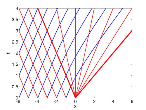
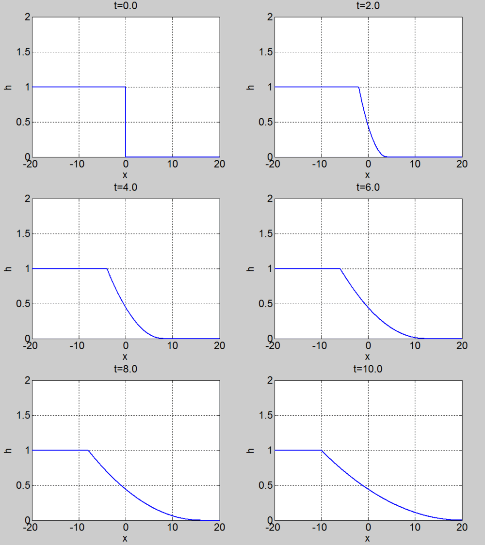
The dam break problem
Assume the water occupies the region
On the characteristic that originates at
where
Therefore, if a
and hence,
so these characteristics are straight lines in the region
The
and on each of the
Since the fluid occupies
which in turn implies that
We also have
Where we have assumed that, since
It remains to determine the
When
and substituting the solution we found for
Solving this ODE subject to
the equation for a characteristic curve.
The curves indeed fill the domain
| Characteristics | Surface elevation |
|---|---|
Shocks
For a unique solution two exist there must be a single
Accelerating Piston
We now consider the problem of water initially at rest occupying the
half space
We assume that the
and this condition must hold throughout the fluid.
On the
The
where
On the
Hence
using the condition
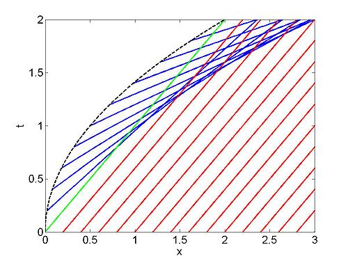
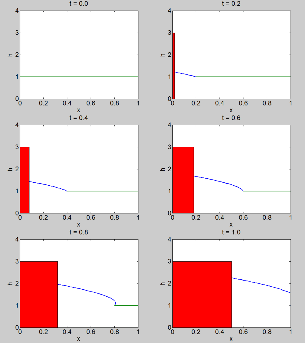
It follows that neighbouring characteristics will meet when
which implies that
The first time that a shock forms is the minimum value of this equation.
For this piston example, this occurs when
| Characteristics | Surface elevation |
|---|---|
Piston Moving with Constant Velocity
This example is also known as the Moving Wall Problem, and is connected to Shallow Water Bores.
We consider the case of a piston, with positive constant velocity
The
and the
so that these two characteristics will intersect at
Speed of the shock
We need the conservation equations in integral form to determine the speed of the shock. Conservation of mass, written as an integral is
If the shock is located at
where
where
We now need to consider the equation for conservation of momentum. In integral form this is
where the pressure
(i.e. we have hydrostatic equilibrium). We can apply a similar argument as before to obtain
Hydraulic Jump
For a hydraulic jump,
If we introduce the variables
and
where
This expression has the roots
The only physically meaningful solution is the root which satisfies
Below is a video of a hydraulic jump. You can clearly see the point where the flow is changing from supercritical to subcritical (look for the small turbulent region in the channel)
Shallow Water Bore
We now consider a bore, in which
the shock wave advances into still water.
We denote the fluid speed by
and
which can be solved to obtain the shock speed and the height of the moving fluid.
Below is a video of surfing on the Severn bore, do not believe everything they say. You might also want to check out the Pororoca a tidal bore on the Amazon.


