Difference between revisions of "Example Calculations for the KdV and IST"
(Created page with '{{nonlinear waves course | chapter title = Example Calculations for the KdV and IST | next chapter = Connection betwen KdV and the Schrodinger Equation | previous chapter …') |
|||
| (11 intermediate revisions by the same user not shown) | |||
| Line 1: | Line 1: | ||
{{nonlinear waves course | {{nonlinear waves course | ||
| chapter title = Example Calculations for the KdV and IST | | chapter title = Example Calculations for the KdV and IST | ||
| − | | next chapter = [[ | + | | next chapter = [[Reaction-Diffusion Systems]] |
| − | | previous chapter = [[ | + | | previous chapter = [[Connection betwen KdV and the Schrodinger Equation]] |
}} | }} | ||
| − | ==Example1 | + | We consider here the two examples we treated in [[Properties of the Linear Schrodinger Equation]]. |
| + | |||
| + | ==Example1: <math>\delta</math> function potential== | ||
We have already calculated the scattering data for the delta function | We have already calculated the scattering data for the delta function | ||
| − | potential. The | + | potential in [[Properties of the Linear Schrodinger Equation]]. The scattering data is |
<center><math> | <center><math> | ||
S\left( \lambda,0\right) =\left( k_{1},\sqrt{k_{1}},\frac{u_{0}}{2ik-u_{0} | S\left( \lambda,0\right) =\left( k_{1},\sqrt{k_{1}},\frac{u_{0}}{2ik-u_{0} | ||
| Line 33: | Line 35: | ||
</math></center> | </math></center> | ||
| − | + | ==Example 2: Hat Function Potential== | |
| − | ==Example 2 | ||
We solve for the case when | We solve for the case when | ||
| Line 40: | Line 41: | ||
u\left( x\right) =\left\{ | u\left( x\right) =\left\{ | ||
\begin{matrix} | \begin{matrix} | ||
| − | |||
0, & x\notin\left[ -1,1\right] \\ | 0, & x\notin\left[ -1,1\right] \\ | ||
20, & x\in\left[ -1,1\right] | 20, & x\in\left[ -1,1\right] | ||
| Line 46: | Line 46: | ||
\right. | \right. | ||
</math></center> | </math></center> | ||
| − | + | We have already solved this case in [[Properties of the Linear Schrodinger Equation]]. | |
| + | For the even solutions we need to solve | ||
<center><math> | <center><math> | ||
\tan\kappa=\frac{k}{\kappa} | \tan\kappa=\frac{k}{\kappa} | ||
</math></center> | </math></center> | ||
| − | + | where <math>\kappa=\sqrt{b-k^{2}}</math>. | |
| + | |||
| + | For the odd solutions we need to solve and | ||
<center><math> | <center><math> | ||
\tan\kappa=-\frac{\kappa}{k} | \tan\kappa=-\frac{\kappa}{k} | ||
</math></center> | </math></center> | ||
| − | |||
Recall that the solitons have amplitude <math>2k_{n}^{2}</math> or <math>-2\lambda_{n}</math>. This | Recall that the solitons have amplitude <math>2k_{n}^{2}</math> or <math>-2\lambda_{n}</math>. This | ||
| Line 65: | Line 67: | ||
<center><math> | <center><math> | ||
u\left( x\right) =\frac{20}{2}\left( \tanh\left( \nu\left( x+1\right) | u\left( x\right) =\frac{20}{2}\left( \tanh\left( \nu\left( x+1\right) | ||
| − | \right) -\tanh\left( \nu\left( x | + | \right) -\tanh\left( \nu\left( x-1\right) \right) \right) |
</math></center> | </math></center> | ||
where <math>\nu</math> is an appropriate constant to make the function increase in value | where <math>\nu</math> is an appropriate constant to make the function increase in value | ||
sufficiently rapidly but not too rapidly. | sufficiently rapidly but not too rapidly. | ||
| + | |||
| + | |||
| + | |||
| + | {| class="wikitable" | ||
| + | |- | ||
| + | ! Animation | ||
| + | ! Three-dimensional plot. | ||
| + | |- | ||
| + | | [[Image:Wide_function.gif|thumb|right|500px|Evolution of <math>u(x,t)</math>.]] | ||
| + | | [[Image:Widefunction.jpg|thumb|right|500px|Evolution of <math>u(x,t)</math> ]] | ||
| + | |||
| + | |} | ||
| + | |||
| + | == Lecture Videos == | ||
| + | |||
| + | === Part 1 === | ||
| + | |||
| + | {{#ev:youtube|K0zeheguRKo}} | ||
Latest revision as of 03:38, 1 October 2020
| Nonlinear PDE's Course | |
|---|---|
| Current Topic | Example Calculations for the KdV and IST |
| Next Topic | Reaction-Diffusion Systems |
| Previous Topic | Connection betwen KdV and the Schrodinger Equation |
We consider here the two examples we treated in Properties of the Linear Schrodinger Equation.
Example1: [math]\displaystyle{ \delta }[/math] function potential
We have already calculated the scattering data for the delta function potential in Properties of the Linear Schrodinger Equation. The scattering data is
The spectral data evolves as
so that
Example 2: Hat Function Potential
We solve for the case when
We have already solved this case in Properties of the Linear Schrodinger Equation. For the even solutions we need to solve
where [math]\displaystyle{ \kappa=\sqrt{b-k^{2}} }[/math].
For the odd solutions we need to solve and
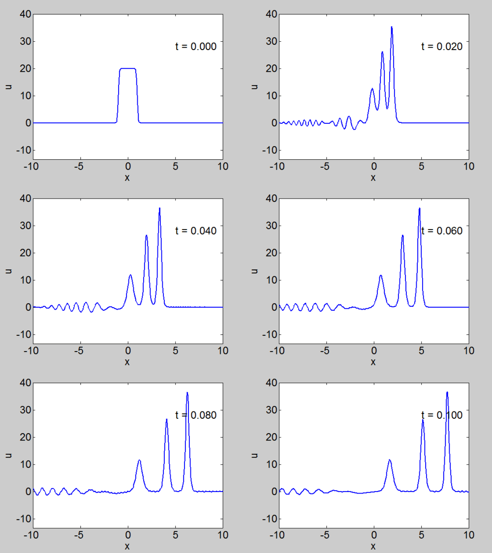
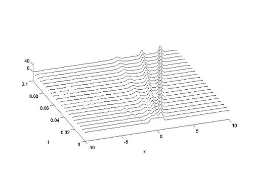
Recall that the solitons have amplitude [math]\displaystyle{ 2k_{n}^{2} }[/math] or [math]\displaystyle{ -2\lambda_{n} }[/math]. This can be seen in the height of the solitary waves.
We cannot work with a hat function numerically, because the jump in [math]\displaystyle{ u }[/math] leads to high frequencies which dominate the response.. We can smooth our function by a number of methods. We use here the function [math]\displaystyle{ \tanh\left( x\right) }[/math] so we write
where [math]\displaystyle{ \nu }[/math] is an appropriate constant to make the function increase in value sufficiently rapidly but not too rapidly.
| Animation | Three-dimensional plot. |
|---|---|

