Example Calculations for the KdV and IST

Nonlinear PDE's Course
Current Topic	Example Calculations for the KdV and IST
Next Topic	Connection betwen KdV and the Schrodinger Equation
Previous Topic	Reaction-Diffusion Systems

Example1 Delta function potential.

We have already calculated the scattering data for the delta function potential. The scattering data is

[math]\displaystyle{ S\left( \lambda,0\right) =\left( k_{1},\sqrt{k_{1}},\frac{u_{0}}{2ik-u_{0} },\frac{2ik}{2ik-u_{0}}\right) }[/math]

The spectral data evolves as

[math]\displaystyle{ k_{1}=k_{1} }[/math] [math]\displaystyle{ c_{1}\left( t\right) =c_{1}\left( 0\right) e^{4k_{1}^{3}t}=\sqrt{k_{1} }e^{4k_{1}^{3}t} }[/math] [math]\displaystyle{ r\left( k,t\right) =r\left( k,0\right) e^{8ik^{3}t} }[/math] [math]\displaystyle{ a\left( k,t\right) =a\left( k,0\right) }[/math]

so that

[math]\displaystyle{ S\left( \lambda,t\right) =\left( k_{1},\sqrt{k_{1}}e^{4k_{1}^{3}t} ,\frac{u_{0}}{2ik-u_{0}}e^{8ik^{3}t},\frac{2ik}{2ik-u_{0}}\right) }[/math]

Example 2 A Hat Function

We solve for the case when

[math]\displaystyle{ u\left( x\right) =\left\{ \begin{matrix} 0, & x\notin\left[ -1,1\right] \\ 20, & x\in\left[ -1,1\right] \end{matrix} \right. }[/math]

For the even solutions we need to solve

[math]\displaystyle{ \tan\kappa=\frac{k}{\kappa} }[/math]

where [math]\displaystyle{ \kappa=\sqrt{b-k^{2}} }[/math].

For the odd solutions we need to solve and

[math]\displaystyle{ \tan\kappa=-\frac{\kappa}{k} }[/math]

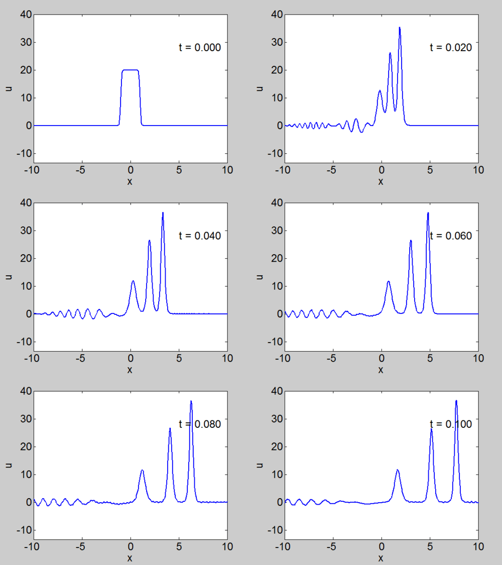
Recall that the solitons have amplitude [math]\displaystyle{ 2k_{n}^{2} }[/math] or [math]\displaystyle{ -2\lambda_{n} }[/math]. This can be seen in the height of the solitary waves.

We cannot work with a hat function numerically, because the jump in [math]\displaystyle{ u }[/math] leads to high frequencies which dominate the response.. We can smooth our function by a number of methods. We use here the function [math]\displaystyle{ \tanh\left( x\right) }[/math] so we write

[math]\displaystyle{ u\left( x\right) =\frac{20}{2}\left( \tanh\left( \nu\left( x+1\right) \right) -\tanh\left( \nu\left( x+1\right) \right) \right) }[/math]

where [math]\displaystyle{ \nu }[/math] is an appropriate constant to make the function increase in value sufficiently rapidly but not too rapidly.

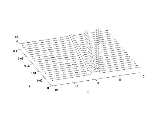
Animation	Three-dimensional plot.
Evolution of [math]\displaystyle{ u(x,t) }[/math].	Evolution of [math]\displaystyle{ u(x,t) }[/math]