|
|
| Line 220: |
Line 220: |
| | 2\nu }\right] \mathrm{d}y} | | 2\nu }\right] \mathrm{d}y} |
| | \end{matrix}</math></center> | | \end{matrix}</math></center> |
| | + | |
| | + | == Lecture Videos == |
| | + | |
| | + | === Part 1 === |
| | + | |
| | + | {{#ev:youtube|tVXQmxOG_6Y}} |
| | + | |
| | + | === Part 2 === |
| | + | |
| | + | {{#ev:youtube|hzgpMM_wWts}} |
| | + | |
| | + | === Part 3 === |
| | + | |
| | + | {{#ev:youtube|uH4B1XsGB-0}} |
| | + | |
| | + | === Part 4 === |
| | + | |
| | + | {{#ev:youtube|h6aDmCtJygM}} |
| | + | |
| | + | === Part 5 === |
| | + | |
| | + | {{#ev:youtube|CsnUKrLjtyQ}} |
Latest revision as of 02:14, 24 October 2020
Introduction
We have already met the conservation law for the traffic equations
[math]\displaystyle{
\partial _{t}\rho +c\left( \rho \right) \partial _{x}\rho =0
}[/math]
and seen how this leads to shocks. We can smooth this equation by adding
dispersion to the equation to give us
[math]\displaystyle{
\partial _{t}\rho +c\left( \rho \right) \partial _{x}\rho =\nu \partial
_{x}^{2}\rho
}[/math]
where [math]\displaystyle{ \nu \gt 0. }[/math]
The simplest equation of this type is to write
[math]\displaystyle{
\partial _{t}u+u\partial _{x}u=\nu \partial _{x}^{2}u
}[/math]
(changing variables to [math]\displaystyle{ u }[/math] and this equation is known as Burgers equation.
Travelling Wave Solution
We can find a travelling wave solution by assuming that
[math]\displaystyle{
u\left( x,t\right) =u\left( x-ct\right) =u\left( \xi \right)
}[/math]
This leads to the equations
[math]\displaystyle{
-cu^{\prime }+u^{\prime }u-\nu u^{\prime \prime }=0
}[/math]
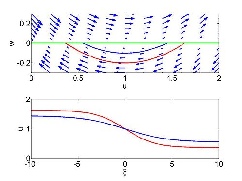
We begin by looking at the phase plane for this system, writing [math]\displaystyle{ w=u^{\prime
} }[/math] so that
[math]\displaystyle{ \begin{matrix}
\dfrac{\mathrm{d}u}{\mathrm{d}\xi } &=&w \\
\dfrac{\mathrm{d}w}{\mathrm{d}\xi } &=&\frac{1}{\nu }\left( w\left( u-c\right) \right)
\end{matrix} }[/math]
This is a degenerate system with the entire [math]\displaystyle{ u }[/math] axis being equilibria.
We can also solve this equation exactly as follows.
[math]\displaystyle{
-cu^{\prime }+u^{\prime }u-\nu u^{\prime \prime }=0
}[/math]
can be integrated to give
[math]\displaystyle{
-cu+\frac{1}{2}\left( u\right) ^{2}-\nu u^{\prime} =c_{1}
}[/math]
which can be rearranged to give
[math]\displaystyle{
u^{\prime }=\frac{1}{2\nu }\left( \left( u\right) ^{2}-2cu-2c_{1}\right)
}[/math]
We define the two roots of the quadratic [math]\displaystyle{ \left( u\right) ^{2}-2\nu
u-2c_{1}=0 }[/math] by [math]\displaystyle{ u_{1} }[/math] and [math]\displaystyle{ u_{2} }[/math]
and we assume that [math]\displaystyle{ u_{2} \lt u_{1} }[/math]. Note that there is only a bounded
solution if we have two real roots and for the bounded solution
[math]\displaystyle{ u_{2} \lt u \lt u_{1} }[/math].
We note that the wave speed
is
[math]\displaystyle{
c=\frac{1}{2}\left( u_{1}+u_{2}\right)
}[/math]
The equation can therefore be written as
[math]\displaystyle{
2\nu u^{\prime }=\left( u-u_{1}\right) \left( u-u_{2}\right)
}[/math]
which has solution
[math]\displaystyle{
u\left( \xi \right) =\frac{1}{2}\left( u_{1}+u_{2}\right) -\frac{1}{2}\left(
u_{1}-u_{2}\right) \tanh \left[ \left( \frac{\xi }{4\nu }\right) \left(
u_{1}-u_{2}\right) \right]
}[/math]
Numerical Solution of Burgers equation
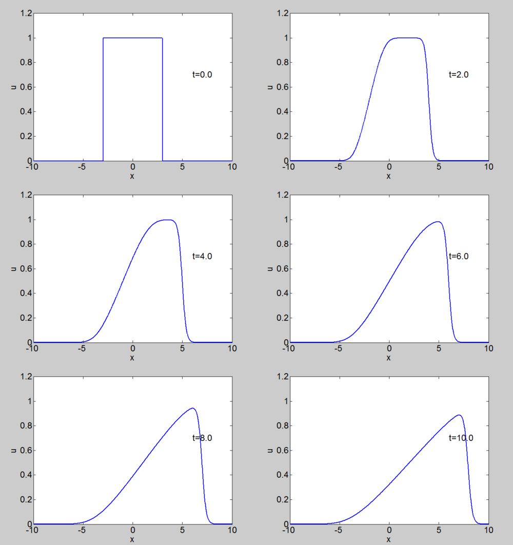
We can solve the equation using our split step spectral method. The equation
can be written as
[math]\displaystyle{
\partial _{t}u=-\frac{1}{2}\partial _{x}\left( u^{2}\right) +\nu \partial
_{x}^{2}u
}[/math]
We solve this by solving in Fourier space to give
[math]\displaystyle{
\partial _{t}\hat{u}=-\frac{1}{2}ik \widehat{\left( u^{2}\right)} -\nu k^{2}\hat{u}
}[/math]
Then we solve each of the steps in turn
for a small time interval to give
[math]\displaystyle{ \begin{matrix}
\tilde{u}\left( k,t+\Delta t\right) &=&\hat{u}\left( k,t\right) -\frac{
\Delta t}{2}ik\mathcal{F}\left( \left[ \mathcal{F}^{-1}\hat{u}\left(
k,t\right) \right] ^{2}\right) \\
\hat{u}\left( k,t+\Delta t\right) &=&\tilde{u}\left( k,t+\Delta t\right)
\exp \left( -\nu k^{2}\Delta t\right)
\end{matrix} }[/math]
| Phase plane for a travelling wave solution
|
Numerical solution of Burgers equation
|
 Phase plane for a travelling wave solution of Burgers equation |
 Numerical solution of Burgers equation |
Exact Solution of Burgers equations
We can find an exact solution to Burgers equation. We want to solve
[math]\displaystyle{ \begin{matrix}
\partial _{t}u+u\partial _{x}u &=&\nu \partial _{x}^{2}u \\
u\left( x,0\right) &=&F\left( x\right)
\end{matrix} }[/math]
Frist we write the equation as
[math]\displaystyle{
\partial _{t}u+\partial _{x}\left( \frac{u^{2}}{2}-\nu \partial _{x}u\right)
=0
}[/math]
We want to find a function [math]\displaystyle{ \psi \left( x,t\right) }[/math] such that
[math]\displaystyle{
\partial _{x}\psi =u,\ \ \partial _{t}\psi =\nu \partial _{x}u-\frac{u^{2}}{2
}
}[/math]
Note that because [math]\displaystyle{ \partial _{x}\partial _{t}\psi =\partial _{t}\partial
_{x}\psi }[/math] we will satisfy Burgers equation. This gives us the following
equation for [math]\displaystyle{ \psi }[/math]
[math]\displaystyle{
\partial _{t}\psi =\nu \partial _{x}^{2}\psi -\frac{1}{2}\left( \partial
_{x}\psi \right) ^{2}
}[/math]
We introduce the Cole-Hopf transformation
[math]\displaystyle{
\psi =-2\nu \log \left( \phi \right)
}[/math]
From this we can obtain the three results:
[math]\displaystyle{
\begin{align}
\partial _{x}\psi &=-2\nu \frac{\partial _{x}\phi }{\phi } \\
\partial _{x}^{2}\psi &=2\nu \left( \frac{\partial _{x}\phi }{\phi }\right)
^{2}-\frac{2\nu }{\phi }\partial _{x}^{2}\phi \\
\partial _{t}\psi &=-2\nu \frac{\partial _{t}\phi }{\phi }
\end{align}
}[/math]
Therefore
[math]\displaystyle{
\partial _{t}\psi =\nu \partial _{x}^{2}\psi -\frac{1}{2}\left( \partial
_{x}\psi \right) ^{2}
}[/math]
becomes
[math]\displaystyle{
-2\nu \frac{\partial _{t}\phi }{\phi }=2\nu ^{2}\left( \frac{\partial
_{x}\phi }{\phi }\right) ^{2}
-2\nu^2 \frac{\partial_x^2\phi}{\phi}
-\frac{1}{2}\left( 2\nu \frac{\partial _{x}\phi
}{\phi }\right) ^{2}
}[/math]
or
[math]\displaystyle{
\partial _{t}\phi =\nu \partial _{x}^{2}\phi
}[/math]
which is just the diffusion equation. Note that we also have to transform the
boundary conditions. We have
[math]\displaystyle{
F\left( x\right) =u\left( x,0\right) =-2\nu \frac{\partial _{x}\phi \left(
x,0\right) }{\phi \left( x,0\right) }
}[/math]
We can write this as
[math]\displaystyle{
\frac{\mathrm{d}}{\mathrm{d}x}\left( \log \left( \phi \right) \right) =-\frac{1}{2\nu }F\left(
x\right)
}[/math]
which has solution
[math]\displaystyle{
\phi \left( x,0\right) =\Phi \left( x\right) =\exp \left( -\frac{1}{2\nu }
\int_{0}^{x}F\left( s\right) \mathrm{d}s\right)
}[/math]
We need to solve
[math]\displaystyle{ \begin{matrix}
\partial _{t}\phi &=&\nu \partial _{x}^{2}\phi \\
\phi \left( x,0\right) &=&\Phi \left( x\right)
\end{matrix} }[/math]
We take the Fourier transform and obtain
[math]\displaystyle{ \begin{matrix}
\partial _{t}\hat{\phi} &=&-k^{2}\nu \hat{\phi} \\
\hat{\phi}\left( k,0\right) &=&\hat{\Phi}\left( k\right)
\end{matrix} }[/math]
which has solution
[math]\displaystyle{
\hat{\phi}\left( k,t\right) =\hat{\Phi}\left( k\right) e^{-k^{2}\nu t}
}[/math]
We can then use the convolution theorem to write
[math]\displaystyle{ \begin{matrix}
\phi \left( x,t\right) &=&\Phi \left( x\right) * \mathcal{F}^{-1}\left[
e^{-k^{2}\nu t}\right] \\
&=&\frac{1}{2\sqrt{\pi \nu t}}\int_{-\infty }^{\infty }\Phi \left( y\right)
\exp \left[ -\frac{\left( x-y\right) ^{2}}{4\nu t}\right] \mathrm{d}y
\end{matrix} }[/math]
Which can be expressed as
[math]\displaystyle{
\phi \left( x,t\right) =\frac{1}{2\sqrt{\pi \nu t}}\int_{-\infty }^{\infty
}\exp \left[ -\frac{f}{2\nu }\right] \mathrm{d}y
}[/math]
where
[math]\displaystyle{
f\left( x,y,t\right) =\frac{1}{2\nu }\int_{0}^{y}F\left( s\right) \mathrm{d}s+\frac{
\left( x-y\right) ^{2}}{2t}
}[/math]
To find [math]\displaystyle{ u }[/math] we recall that
[math]\displaystyle{ \begin{matrix}
u\left( x,t\right) &=&-2\nu \dfrac{\partial _{x}\phi \left( x,t\right) }{\phi
\left( x,t\right) } \\
&=&\dfrac{\int_{-\infty }^{\infty }\left( \frac{x-y}{t}\right) \exp \left[ -
\dfrac{f}{2\nu }\right] \mathrm{d}y}{\int_{-\infty }^{\infty }\exp \left[ -\frac{f}{
2\nu }\right] \mathrm{d}y}
\end{matrix} }[/math]
Lecture Videos
Part 1
Part 2
Part 3
Part 4
Part 5

