The printable version is no longer supported and may have rendering errors. Please update your browser bookmarks and please use the default browser print function instead.
Introduction
We have already met the conservation law for the traffic equations
[math]\displaystyle{
\partial _{t}\rho +c\left( \rho \right) \partial _{x}\rho =0
}[/math]
and seen how this leads to shocks. We can smooth this equation by adding
dispersion to the equation to give us
[math]\displaystyle{
\partial _{t}\rho +c\left( \rho \right) \partial _{x}\rho =\nu \partial
_{x}^{2}\rho
}[/math]
where [math]\displaystyle{ \nu \gt 0. }[/math]
The simplest equation of this type is to write
[math]\displaystyle{
\partial _{t}u+u\partial _{x}u=\nu \partial _{x}^{2}u
}[/math]
(changing variables to [math]\displaystyle{ u }[/math] and this equation is known as Burgers equation.
Travelling Wave Solution
We can find a travelling wave solution by assuming that
[math]\displaystyle{
u\left( x,t\right) =u\left( x-ct\right) =u\left( \xi \right)
}[/math]
This leads to the equations
[math]\displaystyle{
-cu^{\prime }+u^{\prime }u-\nu u^{\prime \prime }=0
}[/math]
We begin by looking at the phase plane for this system, writing [math]\displaystyle{ w=u^{\prime
} }[/math] so that
[math]\displaystyle{ \begin{matrix}
\dfrac{\mathrm{d}u}{\mathrm{d}\xi } &=&w \\
\dfrac{\mathrm{d}w}{\mathrm{d}\xi } &=&\frac{1}{\nu }\left( w\left( u-c\right) \right)
\end{matrix} }[/math]
This is a degenerate system with the entire [math]\displaystyle{ u }[/math] axis being equilibria.
We can also solve this equation exactly as follows.
[math]\displaystyle{
-cu^{\prime }+u^{\prime }u-\nu u^{\prime \prime }=0
}[/math]
can be integrated to give
[math]\displaystyle{
-cu+\frac{1}{2}\left( u\right) ^{2}-\nu u^{\prime} =c_{1}
}[/math]
which can be rearranged to give
[math]\displaystyle{
u^{\prime }=\frac{1}{2\nu }\left( \left( u\right) ^{2}-2cu-2c_{1}\right)
}[/math]
We define the two roots of the quadratic [math]\displaystyle{ \left( u\right) ^{2}-2\nu
u-2c_{1}=0 }[/math] by [math]\displaystyle{ u_{1} }[/math] and [math]\displaystyle{ u_{2} }[/math]
and we assume that [math]\displaystyle{ u_{2} \lt u_{1} }[/math]. Note that there is only a bounded
solution if we have two real roots and for the bounded solution
[math]\displaystyle{ u_{2} \lt u \lt u_{1} }[/math].
We note that the wave speed
is
[math]\displaystyle{
c=\frac{1}{2}\left( u_{1}+u_{2}\right)
}[/math]
The equation can therefore be written as
[math]\displaystyle{
2\nu u^{\prime }=\left( u-u_{1}\right) \left( u-u_{2}\right)
}[/math]
which has solution
[math]\displaystyle{
u\left( \xi \right) =\frac{1}{2}\left( u_{1}+u_{2}\right) -\frac{1}{2}\left(
u_{1}-u_{2}\right) \tanh \left[ \left( \frac{\xi }{4\nu }\right) \left(
u_{1}-u_{2}\right) \right]
}[/math]
Numerical Solution of Burgers equation
We can solve the equation using our split step spectral method. The equation
can be written as
[math]\displaystyle{
\partial _{t}u=-\frac{1}{2}\partial _{x}\left( u^{2}\right) +\nu \partial
_{x}^{2}u
}[/math]
We solve this by solving in Fourier space to give
[math]\displaystyle{
\partial _{t}\hat{u}=-\frac{1}{2}ik \widehat{\left( u^{2}\right)} -\nu k^{2}\hat{u}
}[/math]
Then we solve each of the steps in turn
for a small time interval to give
[math]\displaystyle{ \begin{matrix}
\tilde{u}\left( k,t+\Delta t\right) &=&\hat{u}\left( k,t\right) -\frac{
\Delta t}{2}ik\mathcal{F}\left( \left[ \mathcal{F}^{-1}\hat{u}\left(
k,t\right) \right] ^{2}\right) \\
\hat{u}\left( k,t+\Delta t\right) &=&\tilde{u}\left( k,t+\Delta t\right)
\exp \left( -\nu k^{2}\Delta t\right)
\end{matrix} }[/math]
| Phase plane for a travelling wave solution
|
Numerical solution of Burgers equation
|
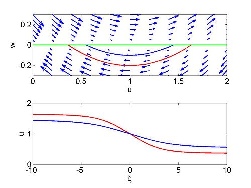 Phase plane for a travelling wave solution of Burgers equation |
 Numerical solution of Burgers equation |
Exact Solution of Burgers equations
We can find an exact solution to Burgers equation. We want to solve
[math]\displaystyle{ \begin{matrix}
\partial _{t}u+u\partial _{x}u &=&\nu \partial _{x}^{2}u \\
u\left( x,0\right) &=&F\left( x\right)
\end{matrix} }[/math]
Frist we write the equation as
[math]\displaystyle{
\partial _{t}u+\partial _{x}\left( \frac{u^{2}}{2}-\nu \partial _{x}u\right)
=0
}[/math]
We want to find a function [math]\displaystyle{ \psi \left( x,t\right) }[/math] such that
[math]\displaystyle{
\partial _{x}\psi =u,\ \ \partial _{t}\psi =\nu \partial _{x}u-\frac{u^{2}}{2
}
}[/math]
Note that because [math]\displaystyle{ \partial _{x}\partial _{t}\psi =\partial _{t}\partial
_{x}\psi }[/math] we will satisfy Burgers equation. This gives us the following
equation for [math]\displaystyle{ \psi }[/math]
[math]\displaystyle{
\partial _{t}\psi =\nu \partial _{x}^{2}\psi -\frac{1}{2}\left( \partial
_{x}\psi \right) ^{2}
}[/math]
We introduce the Cole-Hopf transformation
[math]\displaystyle{
\psi =-2\nu \log \left( \phi \right)
}[/math]
From this we can obtain the three results:
[math]\displaystyle{
\begin{align}
\partial _{x}\psi &=-2\nu \frac{\partial _{x}\phi }{\phi } \\
\partial _{x}^{2}\psi &=2\nu \left( \frac{\partial _{x}\phi }{\phi }\right)
^{2}-\frac{2\nu }{\phi }\partial _{x}^{2}\phi \\
\partial _{t}\psi &=-2\nu \frac{\partial _{t}\phi }{\phi }
\end{align}
}[/math]
Therefore
[math]\displaystyle{
\partial _{t}\psi =\nu \partial _{x}^{2}\psi -\frac{1}{2}\left( \partial
_{x}\psi \right) ^{2}
}[/math]
becomes
[math]\displaystyle{
-2\nu \frac{\partial _{t}\phi }{\phi }=2\nu ^{2}\left( \frac{\partial
_{x}\phi }{\phi }\right) ^{2}
-2\nu^2 \frac{\partial_x^2\phi}{\phi}
-\frac{1}{2}\left( 2\nu \frac{\partial _{x}\phi
}{\phi }\right) ^{2}
}[/math]
or
[math]\displaystyle{
\partial _{t}\phi =\nu \partial _{x}^{2}\phi
}[/math]
which is just the diffusion equation. Note that we also have to transform the
boundary conditions. We have
[math]\displaystyle{
F\left( x\right) =u\left( x,0\right) =-2\nu \frac{\partial _{x}\phi \left(
x,0\right) }{\phi \left( x,0\right) }
}[/math]
We can write this as
[math]\displaystyle{
\frac{\mathrm{d}}{\mathrm{d}x}\left( \log \left( \phi \right) \right) =-\frac{1}{2\nu }F\left(
x\right)
}[/math]
which has solution
[math]\displaystyle{
\phi \left( x,0\right) =\Phi \left( x\right) =\exp \left( -\frac{1}{2\nu }
\int_{0}^{x}F\left( s\right) \mathrm{d}s\right)
}[/math]
We need to solve
[math]\displaystyle{ \begin{matrix}
\partial _{t}\phi &=&\nu \partial _{x}^{2}\phi \\
\phi \left( x,0\right) &=&\Phi \left( x\right)
\end{matrix} }[/math]
We take the Fourier transform and obtain
[math]\displaystyle{ \begin{matrix}
\partial _{t}\hat{\phi} &=&-k^{2}\nu \hat{\phi} \\
\hat{\phi}\left( k,0\right) &=&\hat{\Phi}\left( k\right)
\end{matrix} }[/math]
which has solution
[math]\displaystyle{
\hat{\phi}\left( k,t\right) =\hat{\Phi}\left( k\right) e^{-k^{2}\nu t}
}[/math]
We can then use the convolution theorem to write
[math]\displaystyle{ \begin{matrix}
\phi \left( x,t\right) &=&\Phi \left( x\right) * \mathcal{F}^{-1}\left[
e^{-k^{2}\nu t}\right] \\
&=&\frac{1}{2\sqrt{\pi \nu t}}\int_{-\infty }^{\infty }\Phi \left( y\right)
\exp \left[ -\frac{\left( x-y\right) ^{2}}{4\nu t}\right] \mathrm{d}y
\end{matrix} }[/math]
Which can be expressed as
[math]\displaystyle{
\phi \left( x,t\right) =\frac{1}{2\sqrt{\pi \nu t}}\int_{-\infty }^{\infty
}\exp \left[ -\frac{f}{2\nu }\right] \mathrm{d}y
}[/math]
where
[math]\displaystyle{
f\left( x,y,t\right) =\frac{1}{2\nu }\int_{0}^{y}F\left( s\right) \mathrm{d}s+\frac{
\left( x-y\right) ^{2}}{2t}
}[/math]
To find [math]\displaystyle{ u }[/math] we recall that
[math]\displaystyle{ \begin{matrix}
u\left( x,t\right) &=&-2\nu \dfrac{\partial _{x}\phi \left( x,t\right) }{\phi
\left( x,t\right) } \\
&=&\dfrac{\int_{-\infty }^{\infty }\left( \frac{x-y}{t}\right) \exp \left[ -
\dfrac{f}{2\nu }\right] \mathrm{d}y}{\int_{-\infty }^{\infty }\exp \left[ -\frac{f}{
2\nu }\right] \mathrm{d}y}
\end{matrix} }[/math]
Lecture Videos
Part 1
Part 2
Part 3
Part 4
Part 5

