Method of Characteristics for Linear Equations

Nonlinear PDE's Course
Current Topic	Method of Characteristics for Linear Equations
Next Topic	Traffic Waves
Previous Topic

This is a complete page

We present here a brief account of the method of characteristic for linear waves.

Introduction

The method of characteristics is an important method for hyperbolic PDE's which applies to both linear and nonlinear equations.

We begin with the simplest wave equation

[math]\displaystyle{ \partial_t u + \partial_x u = 0,\,\,-\infty \lt x \lt \infty,\,\,t\gt 0, }[/math]

subject to the initial conditions

[math]\displaystyle{ \left. u \right|_{t=0} = f(x) }[/math]

We consider the solution along the curve [math]\displaystyle{ (x,t) = (X(t),t) }[/math]. We then have

[math]\displaystyle{ \frac{\mathrm{d} }{\mathrm{d} t} u(X(t),t) = \partial_t u + \frac{\mathrm{d} X}{\mathrm{d}t}\partial_x u = \partial_x u \left(\frac{\mathrm{d} X}{\mathrm{d}t} - 1 \right) }[/math]

Therefore along the curve [math]\displaystyle{ \frac{\mathrm{d} X}{\mathrm{d}t} = 1 }[/math] [math]\displaystyle{ u(x,t) }[/math] must be a constant. These are nothing but the straight lines [math]\displaystyle{ x = t+c }[/math] This means that we have

[math]\displaystyle{ u(x,t) = u(t+c,t) = u(c,0) = f(c) = f(x-t)\, }[/math]

Therefore the solution is [math]\displaystyle{ u(x,t) = f(x-t)\, }[/math].

General Form

If we consider the equation

[math]\displaystyle{ \partial_t u + a(x,t)\partial_x u = 0,\,\,-\infty \lt x \lt \infty,\,\,t\gt 0, }[/math]

then we can apply the method of characteristics. We consider the solution along the curve [math]\displaystyle{ (x,t) = (X(t),t) }[/math]. We then have

[math]\displaystyle{ \frac{\mathrm{d} }{\mathrm{d} t} u(X(t),t) = \partial_t u + \frac{\mathrm{d} X}{\mathrm{d}t}\partial_x u = \partial_x u \left(\frac{\mathrm{d} X}{\mathrm{d}t} - a(x,t) \right). }[/math]

This gives us the following o.d.e. for the characteristic curves (along which the solution is a constant)

[math]\displaystyle{ \frac{\mathrm{d} X}{\mathrm{d} t} = a(x,t) . }[/math]

Example 1

Characteristic for Example 1

Consider the equation

[math]\displaystyle{ \partial_t u + x \partial_x u = 0,\,\,-\infty \lt x \lt \infty,\,\,t\gt 0, }[/math]

subject to the initial conditions

[math]\displaystyle{ \left. u \right|_{t=0} = f(x) }[/math]

We consider the solution along the curve [math]\displaystyle{ (x,t) = (X(t),t) }[/math]. We then have

[math]\displaystyle{ \frac{\mathrm{d} }{\mathrm{d} t} u(X(t),t) = \partial_t u + \frac{\mathrm{d}X}{\mathrm{d}t}\partial_x u = \partial_x u \left(\frac{\mathrm{d} X}{\mathrm{d}t} - x \right) }[/math]

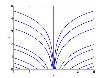
Therefore along the curve [math]\displaystyle{ \frac{\mathrm{d} X}{\mathrm{d}t} = x }[/math] [math]\displaystyle{ u(x,t) }[/math] must be a constant. These are the curves [math]\displaystyle{ x = ce^t }[/math] This means that we have

[math]\displaystyle{ u(x,t) = u(ce^t,t) = u(c,0) = f(c) = f(xe^{-t})\, }[/math]

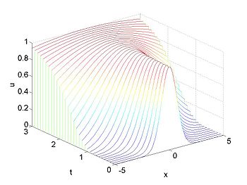
Therefore the solution is given [math]\displaystyle{ u(x,t) = f(xe^{-t})\, }[/math].

Solution for Example 1 with [math]\displaystyle{ f(x) = e^{-x^2} }[/math]

Example 2

Consider the equation

[math]\displaystyle{ \partial_t u + t \partial_x u = 0,\,\,-\infty \lt x \lt \infty,\,\,t\gt 0, }[/math]

subject to the initial conditions

[math]\displaystyle{ \left. u \right|_{t=0} = f(x) }[/math]

We consider the solution along the curve [math]\displaystyle{ (x,t) = (X(t),t) }[/math]. We then have

[math]\displaystyle{ \frac{\mathrm{d} }{\mathrm{d} t} u(X(t),t) = \partial_t u + \frac{\mathrm{d} X}{\mathrm{d}t}\partial_x u = \partial_x u \left(\frac{\mathrm{d} X}{\mathrm{d}t} - t \right) }[/math]

Therefore along the curve [math]\displaystyle{ \frac{\mathrm{d} X}{\mathrm{d}t} = t }[/math] [math]\displaystyle{ u(x,t) }[/math] must be a constant. These are the curves [math]\displaystyle{ x = t^2/2+c }[/math] This means that we have

[math]\displaystyle{ u(x,t) = u(t^2/2 + c,t) = u(c,0) = f(c) = f(x - t^2/2)\, }[/math]

Therefore the solution is given [math]\displaystyle{ u(x,t) = f(x - t^2/2)\, }[/math].

Non-homogeneous Example

We can also use the method of characteristics in the non-homogeneous case. We show this through an example Consider the equation

[math]\displaystyle{ \partial_t u + t \partial_x u = xt,\,\,-\infty \lt x \lt \infty,\,\,t\gt 0, }[/math]

subject to the initial conditions

[math]\displaystyle{ \left. u \right|_{t=0} = f(x) }[/math]

We consider the solution along the curve [math]\displaystyle{ (x,t) = (X(t),t) }[/math]. We then have

[math]\displaystyle{ \frac{\mathrm{d} u}{\mathrm{d} t} = \partial_t u + \frac{\mathrm{d} X}{\mathrm{d}t}\partial_x u = \partial_x u \left(\frac{\mathrm{d}X}{\mathrm{d}t} - t \right) + xt }[/math]

Therefore along the curve [math]\displaystyle{ \frac{\mathrm{d} X}{\mathrm{d}t} = t }[/math] which are the curves [math]\displaystyle{ x = t^2/2+c }[/math]

[math]\displaystyle{ \frac{\mathrm{d}}{\mathrm{d}t}u(x,t) = xt = t^3/2 + c t }[/math]

Therefore

[math]\displaystyle{ u(t^2/2+c,t) = t^4/8 + c t^2/2 + c_2\, }[/math]

Now

[math]\displaystyle{ u(c,0) = c_2 = f(c) }[/math]

Therefore the solution is given [math]\displaystyle{ u(x,t) = t^4/8 + (x -t^2/2) t^2/2 + f(x-t^2/2)\, }[/math] or [math]\displaystyle{ u(x,t) = -t^4/8 + x t^2/2 + f(x-t^2/2)\, }[/math]