Difference between revisions of "Reaction-Diffusion Systems"
| (5 intermediate revisions by 2 users not shown) | |||
| Line 100: | Line 100: | ||
<center> | <center> | ||
<math> | <math> | ||
| − | c(x,t) = \frac{1}{\sqrt{4\pi D t}} \int_{-\infty}^{\infty} c_0(x) e^{(x-s)^2/4Dt} | + | c(x,t) = \frac{1}{\sqrt{4\pi D t}} \int_{-\infty}^{\infty} c_0(x) e^{(x-s)^2/4Dt}\mathrm{d}s |
</math> | </math> | ||
</center> | </center> | ||
| Line 128: | Line 128: | ||
<center> | <center> | ||
<math> | <math> | ||
| − | \hat{c}_n(0) = \frac{1}{2L} \int_{-L}^{L} e^{-\mathrm{i} k_n x} c_0(x) | + | \hat{c}_n(0) = \frac{1}{2L} \int_{-L}^{L} e^{-\mathrm{i} k_n x} c_0(x) \mathrm{d}x |
</math> | </math> | ||
</center> | </center> | ||
| Line 176: | Line 176: | ||
The '''inverse discrete Fourier transform (IDFT)''' is given by | The '''inverse discrete Fourier transform (IDFT)''' is given by | ||
<center> | <center> | ||
| − | <math>c_n = \frac{1}{ | + | <math>c_n = \frac{1}{N} \sum_{m=0}^{N-1} \hat{c}_m e^{2\pi \mathrm{i}mn/N} \quad \quad n = 0,\dots,N-1.</math> |
</center> | </center> | ||
| Line 186: | Line 186: | ||
</math> | </math> | ||
</center> | </center> | ||
| − | + | Note that the choice of where to put the <math>1/N</math> is arbitrary in the definition of FFT and IFFT and | |
| + | does not exactly match here. Of course since it appears once the formula above is correct regardless. | ||
The only difficulty is that we need to define carefully the values of | The only difficulty is that we need to define carefully the values of | ||
<math>k_n</math> | <math>k_n</math> | ||
| Line 313: | Line 314: | ||
so that <math>\alpha + \beta = c_0 + c_1 e^{-vy}</math>. Boundary conditions | so that <math>\alpha + \beta = c_0 + c_1 e^{-vy}</math>. Boundary conditions | ||
are that as <math>y\to\infty </math> <math>\alpha = 1</math> and | are that as <math>y\to\infty </math> <math>\alpha = 1</math> and | ||
| − | <math>\beta = 0</math> | + | <math>\beta = 0</math> and if <math>y\to-\infty</math> then <math>\alpha = 0</math> and |
| − | + | <math>\beta = 1</math>. Therefore <math>\alpha + \beta = 1</math>. | |
This means that, since <math>\alpha \geq 0</math>, we must have | This means that, since <math>\alpha \geq 0</math>, we must have | ||
<math>0\leq \beta \leq 1</math>. | <math>0\leq \beta \leq 1</math>. | ||
| Line 405: | Line 406: | ||
so that <math>k^2 - vk +1 < 0</math>, which is possible provided <math>v\geq 2</math>, for example | so that <math>k^2 - vk +1 < 0</math>, which is possible provided <math>v\geq 2</math>, for example | ||
<math>k = \dfrac{v}{2}</math>. | <math>k = \dfrac{v}{2}</math>. | ||
| + | |||
| + | == Lecture Videos == | ||
| + | |||
| + | === Part 1 === | ||
| + | |||
| + | {{#ev:youtube|rF4X42jP0v8}} | ||
| + | |||
| + | === Part 2 === | ||
| + | |||
| + | {{#ev:youtube|D0NwYlM-uOg}} | ||
| + | |||
| + | === Part 3 === | ||
| + | |||
| + | {{#ev:youtube|5IEZJtJaDHk}} | ||
| + | |||
| + | === Part 4 === | ||
| + | |||
| + | {{#ev:youtube|t_OjTSwVgdo}} | ||
| + | |||
| + | === Part 5 === | ||
| + | |||
| + | {{#ev:youtube|kTHVZaYezLk}} | ||
| + | |||
| + | === Part 6 === | ||
| + | |||
| + | {{#ev:youtube|MVuSg5_sfYI}} | ||
| + | |||
| + | === Part 7 === | ||
| + | |||
| + | {{#ev:youtube|hxKMOHyy6Bw}} | ||
| + | |||
| + | === Part 8 === | ||
| + | |||
| + | {{#ev:youtube|yQ-O2KIqu44}} | ||
| + | |||
| + | |||
| + | |||
[[Category:Simple Nonlinear Waves]] | [[Category:Simple Nonlinear Waves]] | ||
Latest revision as of 23:15, 24 October 2024
| Nonlinear PDE's Course | |
|---|---|
| Current Topic | Reaction-Diffusion Systems |
| Next Topic | Burgers Equation |
| Previous Topic | Example Calculations for the KdV and IST |
We present here a brief theory of reaction diffusion waves.
Law of Mass Action
The law of mass action states that equation rates are proportional to the concentration of reacting species and the ratio in which they combined. It is discussed in detail in Billingham and King 2000. We will present here a few simple examples.
Example 1: Simple Decay
Suppose we have of chemical
with rate
which has solution
where
Example 2: Quadratic Autocatalysis
This example will be important when we consider reaction diffusion problems. We consider the reaction
with rate proportional to
We can solve these equations by observing that
so that
which is separable with solution
and
Note that
Diffusion
The equation for spatially homogeneous diffusion of a chemical with concentration
which is the heat equation. We will consider this in
only one spatial dimension. Consider it on the boundary
where
We can find the inverse transform using convolution and obtain
Solution of the dispersion equation using FFT
We can solve the dispersion equation using the discrete Fourier transform and
its closely related numerical implementation the FFT (Fast Fourier Transform).
We have already met the FFT Numerical Solution of the KdV but we consider it here in more detail.
We consider the concentration
on the finite domain
where
Note that this is not the same solution as we obtained on the infinite domain because
of the boundary conditions on the finite domain. The coefficients
The key to the numerical solution of this equation is the use of the FFT. We begin by discretising the
domain into a series of
We also get
but we know that
The discrete Fourier transform
The
discrete Fourier transform
of a sequence of 2N complex numbers c0, ..., c2N−1 is transformed into the sequence of N complex numbers
We denote the transform by the symbol
The inverse discrete Fourier transform (IDFT) is given by
Therefore we can write
Note that the choice of where to put the
The real power of this method lies with the Fast Fourier Transform
or FFT algorithm. A naive implementation of the discrete Fourier transform above (or its inverse)
will involve order
Reaction Diffusion Equations
We consider an auto catalytic reaction where the chemical species also diffuse. In this case the equations are
We can non-dimensionalise these equations scaling the variables as
So that the equations become
If we choose
then we obtain the system
Solution via split step method
We can solve this equations numerically using a
split step method. We assume
that at time
from
by assuming that
and we do likewise for the equation for
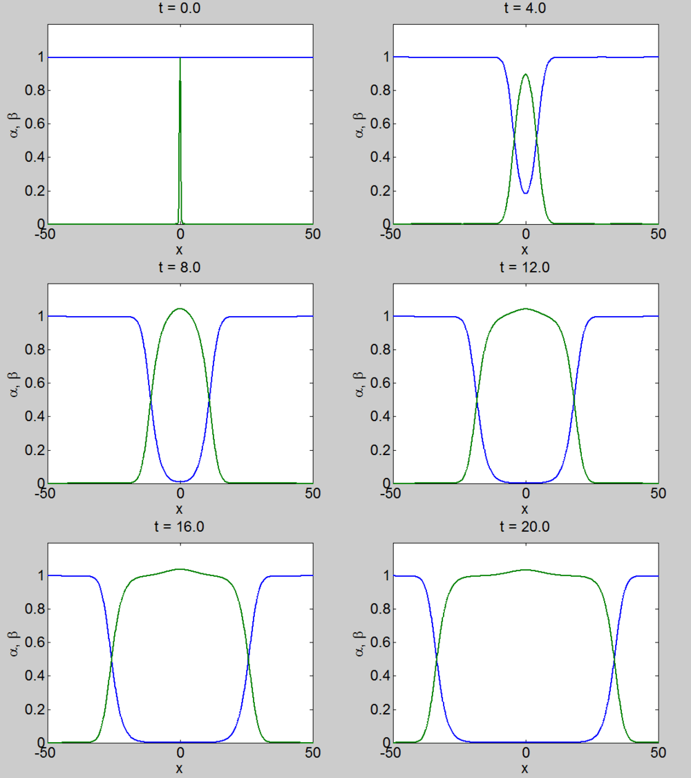
We can easily implement this split step method in matlab and we obtain a pair of travelling waves.
Travelling Waves solution
When we solve the equations we found the solution formed travelling waves and we now consider this phenomena in detail.
We define a new coordinate
and
If we add these equations we obtain
so that
which we can write as the system of first order equations.
We define the variable
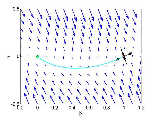
This dynamical system has equilibrium points at
We can easily see that the Jacobian evaluated at our first equilibrium point is
which has eigenvalues
Additionally,
which has eigenvalues
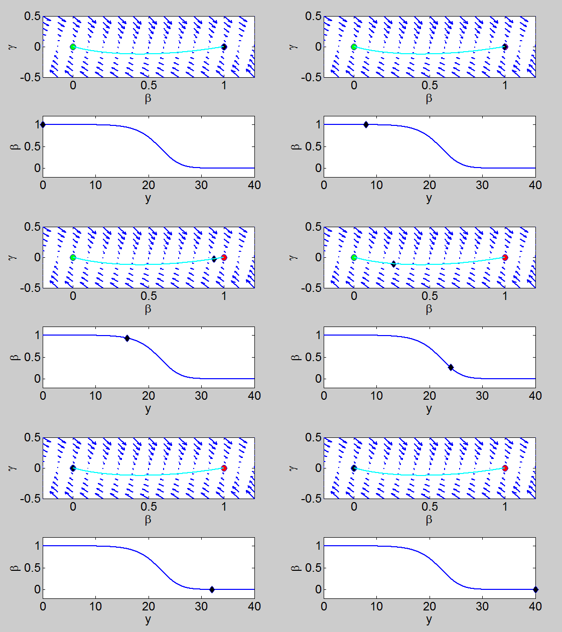
To find a travelling wave we need to find a heteroclinic connection
between the two equilibrium points which also has to satisfy the conditions
that
We need to show that the heteroclinic connection does not cross the
On the line
when


