Traffic Waves

Nonlinear PDE's Course
Current Topic	Traffic Waves
Next Topic	Nonlinear Shallow Water Waves
Previous Topic	Method of Characteristics for Linear Equations

This is a complete page

We consider here some simple equations which model traffic flow. This problem is discussed in Billingham and King 2000.

Equations

We consider a single lane of road, and we measure distance along the road with the variable [math]\displaystyle{ x }[/math] and [math]\displaystyle{ t }[/math] is time. We define the following variables

[math]\displaystyle{ \begin{matrix} &\rho(x,t) &: &\mbox{car density (cars/km)} \\ & v(\rho) &: &\mbox{car velocity (km/hour)} \\ & q(x,t) =\rho v &: &\mbox{car flow rate (cars/hour)} \\ \end{matrix} }[/math]

If we consider a finite length of road [math]\displaystyle{ x_1\leq x \leq x_2 }[/math] then the net flow of cars in and out must be balanced by the change in density. This means that

[math]\displaystyle{ \frac{\partial}{\partial t} \int_{x_1}^{x_2} \rho(x,t) \mathrm{d}x = -q(x_2,t) + q(x_1,t) }[/math]

We now consider continuous densities (which is obviously an approximation) and set [math]\displaystyle{ x_2 = x_1 + \Delta x }[/math] and we obtain

[math]\displaystyle{ \frac{\partial}{\partial t} \rho(x_1,t) = -\frac{q(x_2,t) + q(x_1,t)}{\Delta x} }[/math]

and if we take the limit as [math]\displaystyle{ \Delta x \to 0 }[/math] we obtain the differential equation

[math]\displaystyle{ \frac{\partial \rho}{\partial t} + \frac{\partial q}{\partial x} = 0 }[/math]

Note that this equation has been derived purely from the need to conserve cars (it is a conservation equation) and is not possible to solve this equation until we have derived a connection between [math]\displaystyle{ \rho }[/math] and [math]\displaystyle{ q }[/math].

Equation for [math]\displaystyle{ \rho }[/math] only

At the moment we assume that we have some expression for [math]\displaystyle{ v(\rho) }[/math] If we substitute the expression for [math]\displaystyle{ q = v\rho }[/math] into our differential equation we obtain

[math]\displaystyle{ \frac{\partial \rho}{\partial t} + \frac{\partial }{\partial x} \left(v(\rho)\rho\right) = 0 }[/math]

which gives us

[math]\displaystyle{ \frac{\partial \rho}{\partial t} + \left(v^{\prime}(\rho)\rho + v(\rho)\right) \frac{\partial \rho }{\partial x} = 0 }[/math]

or

[math]\displaystyle{ \frac{\partial \rho}{\partial t} + c(\rho)\frac{\partial \rho }{\partial x} = 0 }[/math]

where [math]\displaystyle{ c(\rho) = \left(v^{\prime}(\rho)\rho + v(\rho)\right) }[/math] is the kinematic wave speed. Note that this is not the speed of the cars, but the speed at which disturbances in the density travel.

A simple relationship between [math]\displaystyle{ \rho }[/math] and [math]\displaystyle{ q }[/math]

The relationship between [math]\displaystyle{ \rho }[/math] and [math]\displaystyle{ q }[/math] is an equation of state and there is no exact equation since it depends on many unknowns. One of the simplest relationship between [math]\displaystyle{ \rho }[/math] and [math]\displaystyle{ q }[/math] is derived from the following assumptions

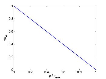
• When the density [math]\displaystyle{ \rho = 0 }[/math] the speed is [math]\displaystyle{ v=v_0 }[/math]
• When the density is [math]\displaystyle{ \rho = \rho_{\max} }[/math] the speed is [math]\displaystyle{ v=0 }[/math]
• The speed is a linear function of [math]\displaystyle{ \rho }[/math] between these two values.

This also gives good fit with measured data. We will either consider the general case or use this simple relationship. Using this we obtain

[math]\displaystyle{ v(\rho) = v_0\frac{\rho_{\max} - \rho}{\rho_{\max}} }[/math]

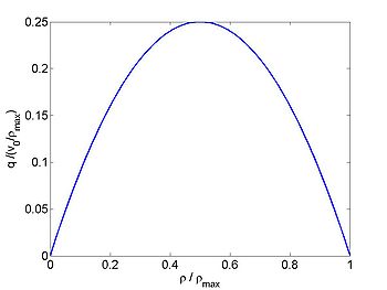
The flux of cars is given by

[math]\displaystyle{ q = \rho v(\rho) = v_0\frac{\rho(\rho_{\max} - \rho)}{\rho_{\max}} }[/math]

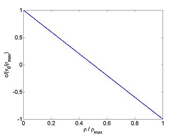
and the wave speed is

[math]\displaystyle{ c(\rho) = \left(v^{\prime}(\rho)\rho + v(\rho)\right) = -\frac{v_0}{\rho_{\max}}\rho + v_0\frac{\rho_{\max} - \rho}{\rho_{\max}} = v_0\frac{\rho_{\max} - 2\rho}{\rho_{\max}} }[/math]

[math]\displaystyle{ v }[/math]	[math]\displaystyle{ q }[/math]	[math]\displaystyle{ c }[/math]
[math]\displaystyle{ v(\rho) }[/math] versus [math]\displaystyle{ \rho }[/math]	[math]\displaystyle{ q(\rho) }[/math] versus [math]\displaystyle{ \rho }[/math]	[math]\displaystyle{ \rho(\rho) }[/math] versus [math]\displaystyle{ \rho }[/math]

Small Amplitude Disturbances

We can linearise the model by assuming that the variation in density is small so that we can write

[math]\displaystyle{ \rho = \rho_0 + \tilde{\rho} }[/math]

where we assume that [math]\displaystyle{ \tilde{\rho} }[/math] is small. This allows us to write the equations as

[math]\displaystyle{ \frac{\partial \tilde{\rho}}{\partial t} + c(\rho_0) \frac{\partial \tilde{\rho}}{\partial x} = 0 }[/math]

where the main difference between this and the full equation is that the wave speed [math]\displaystyle{ c }[/math] is a constant. This is the linearised equation. Note that this linearisation does not give a good model because traffic density does not vary only a small amount about some mean (as is the case for accoustic waves where the density of air is roughly constant).

Under these assumptions the solution to the equation is

[math]\displaystyle{ \tilde{\rho} = f(x - c(\rho_0)t) }[/math]

where [math]\displaystyle{ f }[/math] is determined by the initial condition. This represents disturbances which travel with speed [math]\displaystyle{ c(\rho_0) }[/math] in the positive [math]\displaystyle{ x }[/math] direction.

We now consider the characteristic curves which are curves along which the density [math]\displaystyle{ \rho }[/math] is a constant. These are give by

[math]\displaystyle{ x = X(t) = x_0 + c(\rho_0) t.\, }[/math]

which are just straight lines of constant slope. We will see shortly that the full (nonlinear) equations also possess characteristics.

Nonlinear Initial Value Problem

We wish to solve

[math]\displaystyle{ \frac{\partial \rho}{\partial t} + c(\rho) \frac{\partial \rho}{\partial x} = 0 }[/math]

subject to the initial conditions

[math]\displaystyle{ \rho(x,0) = \rho_0(x) \, }[/math]

It turns out that the concept of characteristic curves is very important for this problem.

If we want [math]\displaystyle{ \rho(X(t),t) }[/math] to be a constant then we require

[math]\displaystyle{ \frac{\mathrm{d}}{\mathrm{d}t}\rho(X(t),t) = \frac{\mathrm{d} X}{\mathrm{d}t} \frac{\partial \rho}{\partial x} + \frac{\partial \rho}{\partial t} = 0. }[/math]

Comparing this to the governing partial differential equation we can see that we require

[math]\displaystyle{ \frac{\mathrm{d} X}{\mathrm{d}t} = c(\rho) }[/math]

This means that the characteristics are straight lines (since [math]\displaystyle{ \rho }[/math] is constant) with slope given by [math]\displaystyle{ c(\rho_0(x_0)) }[/math] so that the equation for the characteristics is

[math]\displaystyle{ X(t) = x_0 + c(\rho_0(x_0))t \, }[/math]

This does not allow us to write down a solution to the initial value problem, all we can do is write

[math]\displaystyle{ \rho(x_0 + c(\rho_0(x_0))t,t) = \rho_0(x_0)\, }[/math]

which allows us to calculate the solution stepping forward in time, but not to determine the solution given a value of [math]\displaystyle{ (x,t) }[/math] (because we have no way of knowing what [math]\displaystyle{ c(\rho_0(x_0)) }[/math] is.

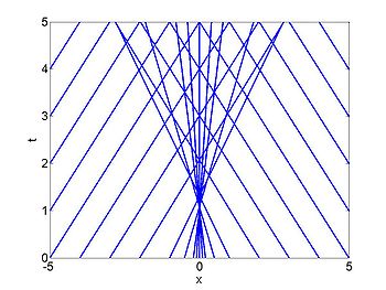
The characteristics are a family of straight lines which will all have different slopes. If two characteristics meet, our solution method will break down because there will be two values of the density [math]\displaystyle{ \rho }[/math]. This gives rise to a shock. It turns out that this the formation of shocks is a product of the equations themselves and not with the solution method. We will see shortly that special methods are required to treat these shocks.

Case when no shocks are formed

The characteristic curves will fill the space without meeting provided that the wave speed [math]\displaystyle{ c(\rho_0) }[/math] is a monotonically increasing function of the distance [math]\displaystyle{ x }[/math]. If we work with our previous model we have

[math]\displaystyle{ v(\rho) = v_0\frac{\rho_{\max} - \rho}{\rho_{\max}} }[/math]

and

[math]\displaystyle{ c(\rho) = v_0\frac{\rho_{\max} - 2\rho}{\rho_{\max}} }[/math]

so that [math]\displaystyle{ c }[/math] is a monotonically decreasing function of density [math]\displaystyle{ \rho }[/math]. This means that the wave speed [math]\displaystyle{ c(\rho_0) }[/math] will be a monotonically increasing function of the distance [math]\displaystyle{ x }[/math] if an only if the density is a monotonically decreasing function. In this case the solution can be calculated straightforwardly by expansion of the initial density.

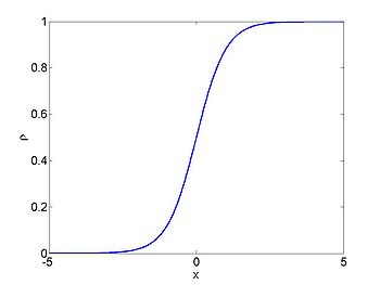
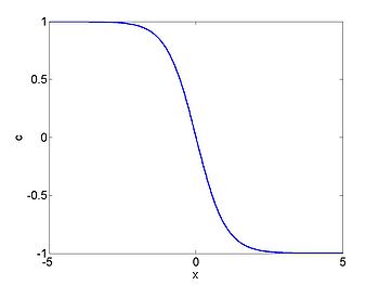
No shock example

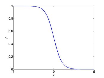
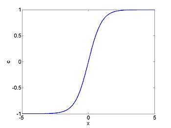
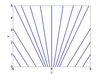
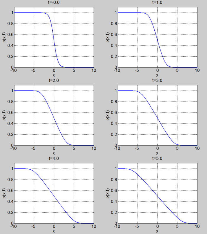
We consider the case when [math]\displaystyle{ \rho_{\max} = v_0 = 1 }[/math] and where the initial density is given by [math]\displaystyle{ \rho_0 = 1/2(1- \tanh(x)) }[/math]. The figures below show the initial density, the initial speed, the characteristics and [math]\displaystyle{ \rho(x,t) }[/math] for this case.

[math]\displaystyle{ \rho }[/math]	[math]\displaystyle{ c }[/math]
[math]\displaystyle{ \rho_0 = 1/2(1- \tanh(x)) }[/math]	[math]\displaystyle{ c(\rho_0) }[/math]

characteristics	[math]\displaystyle{ \rho(x,t) }[/math]
Characterisitics for [math]\displaystyle{ \rho_0 = 1/2(1- \tanh(x)) }[/math]	[math]\displaystyle{ \rho(x,t) for }[/math][math]\displaystyle{ \rho_0 = 1/2(1- \tanh(x)) }[/math]

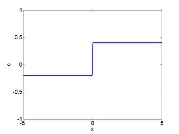
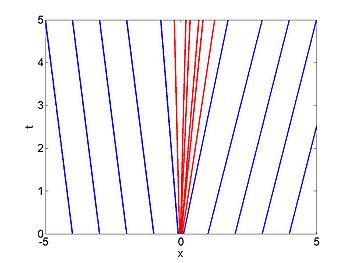
Riemann problem and the expansion fan

We can consider a simple problem in which there is a jump in the initial density

[math]\displaystyle{ \rho(x,0) = \left\{ \begin{matrix} \rho_{L},& x \lt 0 \\ \rho_{R},& x \gt 0 \end{matrix} \right. }[/math]

where [math]\displaystyle{ \rho_{L} \gt \rho_{R} }[/math] so that we do not form a shock. In this case the characteristics on each side of [math]\displaystyle{ x=0 }[/math] have a different slope and the question is what happens between. It is easiest to think about the following problem

[math]\displaystyle{ \rho(x,0) = \left\{ \begin{matrix} \rho_{L},& x \lt -\epsilon \\ \frac{\rho_{R}-\rho_{L}}{2\epsilon}x + \frac{\rho_{R}+\rho_{L}}{2} & -\epsilon \leq x \leq \epsilon \\ \rho_{R},& x \gt \epsilon \end{matrix} \right. }[/math]

We can then see that we have lines of uniformly varying slope for [math]\displaystyle{ -\epsilon\lt x\lt \epsilon }[/math] with slope between [math]\displaystyle{ c(\rho_L) }[/math] and [math]\displaystyle{ c(\rho_R) }[/math]. If we then take the limit as [math]\displaystyle{ \epsilon \to 0 }[/math] we obtain an expansion fan emanating from [math]\displaystyle{ x=0 }[/math].

If we assume that

[math]\displaystyle{ c(\rho) = v_0\frac{\rho_{\max} - 2\rho}{\rho_{\max}} }[/math]

then we know that on the lines of the expansion fan (which all start at [math]\displaystyle{ x=0 }[/math]) we have [math]\displaystyle{ c(\rho) = x/t }[/math]. We can rearrange this and solve for [math]\displaystyle{ x }[/math] and obtain [math]\displaystyle{ \rho =\frac{ 1}{2} \rho_{\max} (1-x/v_0 t) }[/math]

The solution is then given by

[math]\displaystyle{ \rho(x,t) = \left\{ \begin{matrix} \rho_{L},& x \lt c(\rho_L) t\\ \frac{ \rho_{\max}}{2} (1-x/v_0 t),& c(\rho_L) t \leq x \leq c(\rho_R) t\\ \rho_{R},& x \gt c(\rho_R) t \end{matrix} \right. }[/math]

This solution is known as an expansion fan.

We consider the case when [math]\displaystyle{ \rho_{\max} = v_0 = 1 }[/math] and where the initial density is given by

[math]\displaystyle{ \rho(x,0) = \left\{ \begin{matrix} 0.6,& x \lt 0 \\ 0.3,& x \gt 0 \end{matrix} \right. }[/math]

. The figures below show the initial density, the initial speed,

the characteristics and [math]\displaystyle{ \rho(x,t) }[/math] for this case.

[math]\displaystyle{ \rho }[/math]	[math]\displaystyle{ c }[/math]
[math]\displaystyle{ \rho_0 }[/math]	[math]\displaystyle{ c(\rho_0) }[/math]

characteristics	[math]\displaystyle{ \rho(x,t) }[/math]
Characterisitics	File:Expansion fan1.gif [math]\displaystyle{ \rho(x,t) }[/math]

Shocks

So far we have only considered the case when [math]\displaystyle{ c(x_0) }[/math] is monotonically increasing so that two characteristics never cross. We now consider the case when characteristics can meet. A movie of this case is shown below.

We can easily see that the first characteristics to meet will be neighbouring characteristics. Consider two characteristics with

[math]\displaystyle{ X_1(t) = x_0 + c(x_0)t\, }[/math] [math]\displaystyle{ X_2(t) = x_0 + \delta x + c(x_0+\delta x)t\, }[/math]

Then these curves will meet at time [math]\displaystyle{ T }[/math] where

[math]\displaystyle{ x_0 + c(x_0)T = x_0 + \delta x + c(x_0+\delta x)T\, }[/math]

which implies that

[math]\displaystyle{ T = -\frac{1}{c^{\prime}(x_0)} }[/math]

Note the following

• If [math]\displaystyle{ c^{\prime}(x) \gt 0 }[/math] then no shock will form.
• The shock first forms at the minimum positive value of

[math]\displaystyle{ - \frac{1}{c^{\prime}(x)} }[/math] for [math]\displaystyle{ -\infty \lt x \lt \infty }[/math].

Shock Fitting

If we calculate the solution using our formula

[math]\displaystyle{ \rho(x_0 + c(\rho_0(x_0))t,t) = \rho(x_0)\, }[/math]

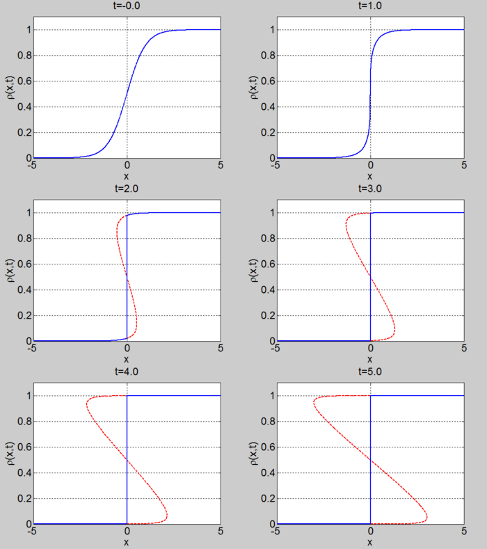
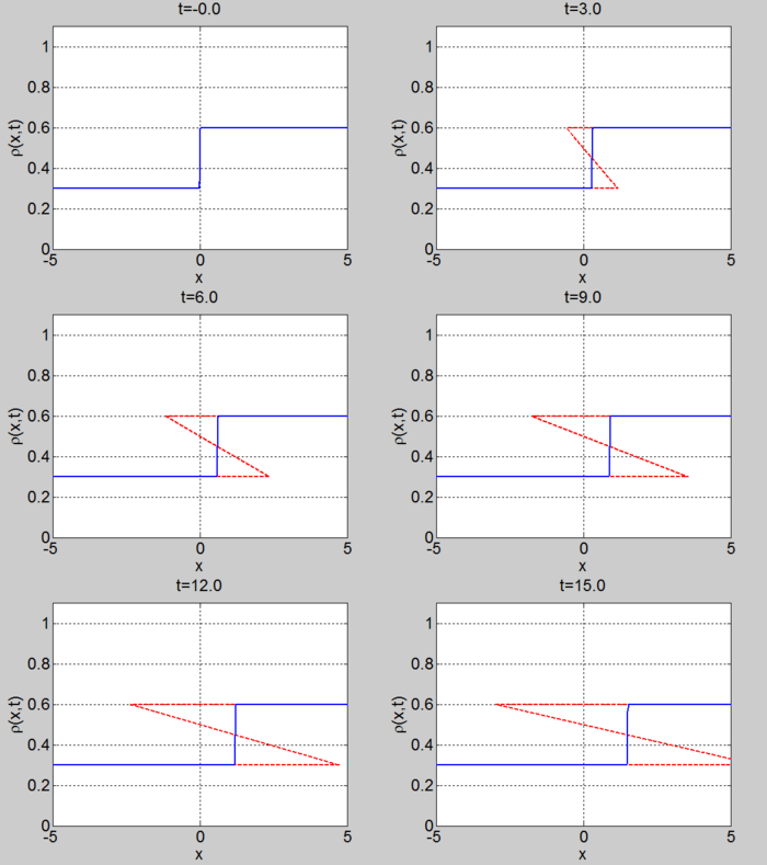
then we find that the solution becomes multivalued in the case when a shock forms. We then have to fit a shock. One way to do this is by imposing the condition that equal areas are removed and added when we chose the position of the shock. This corresponds to the condition that the number of cars must be conserved

Speed of the shock

If we consider the case when there is a shock at [math]\displaystyle{ s(t) }[/math] with [math]\displaystyle{ \rho = \rho^{-} }[/math] at [math]\displaystyle{ x=s^{-} }[/math] and [math]\displaystyle{ \rho = \rho^{+} }[/math] at [math]\displaystyle{ x=s^{+} }[/math] (where [math]\displaystyle{ s^{-} }[/math] is just less than s(t) and [math]\displaystyle{ s^{+} }[/math] is just greater than s(t) ). If we substitute this into the governing integral equation we obtain

[math]\displaystyle{ \frac{\partial}{\partial t} \left( \int_{x_1}^{s(t)} + \int_{s(t)}^{x_2} \rho(x,t)\mathrm{d}x \right) = q(x_1,t) - q(x_2,t) }[/math]

and hence

[math]\displaystyle{ \int_{x_1}^{x_2} \frac{\partial \rho(x,t)}{\partial t} \mathrm{d}x + \frac{\mathrm{d}s}{\mathrm{d}t}\rho^{-} - \frac{\mathrm{d}s}{\mathrm{d}t}\rho^{+} = q(x_1,t) - q(x_2,t) }[/math]

If we now take the limit as [math]\displaystyle{ x_1\to x_2 }[/math] we obtain

[math]\displaystyle{ \frac{\mathrm{d}s}{\mathrm{d}t}\rho^{-} - \frac{\mathrm{d}s}{\mathrm{d}t}\rho^{+} = q(\rho^{-}) - q(\rho^{+}) }[/math]

so that

[math]\displaystyle{ \frac{\mathrm{d}s}{\mathrm{d}t} = \frac{q(\rho^{-}) - q(\rho^{+})} {\rho^{-} - \rho^{+}} }[/math]

Shock example

We consider the case when [math]\displaystyle{ \rho_{\max} = v_0 = 1 }[/math] and where the initial density is given by [math]\displaystyle{ \rho_0 = 1/2(1 + \tanh(x)) }[/math]. The figures below show the initial density, the initial speed, the characteristics and [math]\displaystyle{ \rho(x,t) }[/math] for this case.

[math]\displaystyle{ \rho }[/math]	[math]\displaystyle{ c }[/math]
[math]\displaystyle{ \rho_0 = 1/2(1+ \tanh(x)) }[/math]	[math]\displaystyle{ c(\rho_0) }[/math]

characteristics	[math]\displaystyle{ \rho(x,t) }[/math]
Characterisitics for [math]\displaystyle{ \rho_0 = 1/2(1+ \tanh(x)) }[/math]	[math]\displaystyle{ \rho(x,t) for }[/math][math]\displaystyle{ \rho_0 = 1/2(1+ \tanh(x)) }[/math] Dotted solution is without shock fitting.

Riemann problem

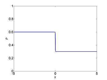
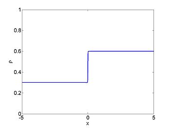
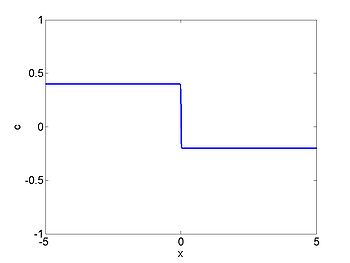
We now consider the Riemann problem

[math]\displaystyle{ \rho(x,0) = \left\{ \begin{matrix} \rho_{L},& x \lt 0 \\ \rho_{R},& x \gt 0 \end{matrix} \right. }[/math]

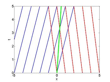
where [math]\displaystyle{ \rho_{L} \lt \rho_{R} }[/math]. In this case a shock forms immediately and the characteristics terminate at the shock. The shock moves with constant speed given by the equation for the motion of the shock (or can be found by the equal areas rule). We obtain

[math]\displaystyle{ \rho(x,t) = \left\{ \begin{matrix} \rho_{L},& x \lt \frac{1}{2} \left(c(\rho_{L}) + c(\rho_{R}) \right) t \\ \rho_{R},& x \gt \frac{1}{2} \left(c(\rho_{L}) + c(\rho_{R}) \right) t \end{matrix} \right. }[/math]

We consider the case when [math]\displaystyle{ \rho_{\max} = v_0 = 1 }[/math] and where the initial density is given by

[math]\displaystyle{ \rho(x,0) = \left\{ \begin{matrix} 0.3,& x \lt 0 \\ 0.6,& x \gt 0 \end{matrix} \right. }[/math]

The figures below show the initial density, the initial speed, the characteristics, and [math]\displaystyle{ \rho(x,t) }[/math] for this case.

[math]\displaystyle{ \rho }[/math]	[math]\displaystyle{ c }[/math]
[math]\displaystyle{ \rho_0 }[/math]	[math]\displaystyle{ c(\rho_0) }[/math]

characteristics	[math]\displaystyle{ \rho(x,t) }[/math]
Characterisitics with shock shown in green.	[math]\displaystyle{ \rho(x,t) }[/math] with the red dotted line showing the solution without shock fitting