|
|
| Line 44: |
Line 44: |
| | | | |
| | | | |
| − | | + | [[Category:Linear Water-Wave Theory]] |
| − | == Solution for the Radiation and Diffracted Potential ==
| |
| − | | |
| − | We use the [[Free-Surface Green Function]] for two-dimensional waves, with singularity at
| |
| − | the water surface since we are only
| |
| − | interested in its value at <math>z=0.</math> Using this we can transform the system of equations to
| |
| − | | |
| − | <center><math>
| |
| − | \phi^{\mathrm{D}}(x) = \phi^{\mathrm{I}}(x) + \int_{-L}^{L}G(x,\xi) \alpha\phi^{\mathrm{S}}(\xi) \mathrm{d} \xi
| |
| − | </math></center>
| |
| − | and
| |
| − | <center><math>
| |
| − | \phi_n^{\mathrm{R}}(x) = \int_{-L}^{L}G(x,\xi)
| |
| − | \left(
| |
| − | \alpha\phi_n^{\mathrm{R}}(\xi) - i\omega X_n(\xi)
| |
| − | \right)\mathrm{d} \xi
| |
| − | </math></center>
| |
| − | | |
| − | Details about this method can be found in [[Integral Equation for the Finite Depth Green Function at Surface]].
| |
| − | | |
| − | == Reflection and Transmission Coefficients ==
| |
| − | | |
| − | The Reflection and Transmission Coefficients represent the ratio of the amplitude of the reflected or transmitted wave to the amplitude of the incident wave. They hold the property that <math> |R|^2+|T|^2=1\,</math> (and may often contain an imaginery element).
| |
| − | | |
| − | [[Image:Square_volume.png|600px|right|thumb|frame|A diagram depicting the area <math>\Omega\,</math> which is bounded by the rectangle <math>\partial \Omega \,</math>. The rectangle <math>\partial \Omega \,</math> is bounded by <math> -h \leq z \leq 0 \,</math> and <math>-\infty \leq x \leq \infty \,</math> or <math>-N \leq x \leq N\,</math>]]
| |
| − | | |
| − | We can calculate the Reflection and Transmission coefficients as follows:
| |
| − | Applying Green's theorem to <math>\phi\,</math> and <math>\phi^{\mathrm{I}}\,</math> gives:
| |
| − | <center><math>
| |
| − | 0 = \iint_{\Omega}(\phi\nabla^2\phi^{\mathrm{I}} - \phi^{\mathrm{I}}\nabla^2\phi)\mathrm{d}x\mathrm{d}z
| |
| − | = \int_{\partial\Omega}(\phi\frac{\partial\phi^{\rm I}}{\partial n} - \phi^{\rm I}\frac{\partial\phi}{\partial n})\mathrm{d}l,
| |
| − | </math></center>
| |
| − | <center><math>
| |
| − | = \phi_0(0) \int_{-L}^{L} e^{k_0 x} \left(\alpha \phi(x) - \partial_n \phi(x)\right)\mathrm{d}x
| |
| − | - 2k_0 R \int_{-h}^{0} \left(\phi_0(z)\right)^2 \mathrm{d}z.
| |
| − | </math></center><br\>
| |
| − | where <math> k_0 \,</math> is the first imaginery root of the dispersion equation and the incident wave is of the form: <math> \phi^I=\phi_0(z)e^{-ikx} \,</math><br\><br\>
| |
| − | Therefore, in the case of a floating plate (where z=0):
| |
| − | <center><math>
| |
| − | R = \frac{\int_{-L}^{L} e^{k_0 x} \left(\alpha \phi(x) - \partial_n \phi(x)\right)\mathrm{d}x }
| |
| − | {2 k_0 \int_{-h}^{0} \left(\phi_0(z)\right)^2 \mathrm{d}z}.
| |
| − | </math></center>
| |
| − | and using a wave incident from the right we obtain
| |
| − | <center><math>
| |
| − | 1 + T = \frac{\int_{-L}^{L} e^{-k_0 x} \left(\alpha \phi(x) - \partial_n \phi(x)\right)\mathrm{d}x }
| |
| − | {2 k_0 \int_{-h}^{0} \left(\phi_0(z)\right)^2 \mathrm{d}z}.
| |
| − | </math></center>
| |
| − | | |
| − | == Matlab Code ==
| |
| − | | |
| − | | |
| − | A program to calculate the solution in elastic modes can be found here
| |
| − | {{elastic plate modes code}}
| |
| − | | |
| − | === Additional code ===
| |
| − | | |
| − | This program requires
| |
| − | * {{green function surface code}}
| |
| − | * {{green function source and field free surface code}}
| |
| − | * {{free surface dispersion equation code}}
| |
| − | * {{eigenvalues beam}}
| |
| − | * {{eigenvectors beam}}
| |
| − | | |
| − | == Alternative Solution Method using Green Functions for a Uniform Plate ==
| |
| − | | |
| − | We can also solve the equation by a closely related method which was given in
| |
| − | [[Meylan and Squire 1994]].
| |
| − | We can transform the equations to
| |
| − | <center><math>
| |
| − | \phi(x) = \phi^{\rm I}(x) + \int_{-L}^{L}G(x,\xi)
| |
| − | \left(
| |
| − | \alpha\phi(\xi) - \partial_z\phi(\xi)
| |
| − | \right)\mathrm{d} \xi
| |
| − | </math></center>
| |
| − | | |
| − | Expanding as before
| |
| − | <center>
| |
| − | <math>
| |
| − | \partial_z \phi = i\omega \sum \xi_n X_n
| |
| − | </math>
| |
| − | </center>
| |
| − | we obtain
| |
| − | <center><math>
| |
| − | -i\omega \phi = \sum \left(\beta\lambda_n^4 - \gamma\alpha + 1\right)\xi_n X_n
| |
| − | </math>
| |
| − | </center>
| |
| − | This leads to the following equation
| |
| − | <center>
| |
| − | <math>
| |
| − | \partial_z\phi(x) = \frac{1}{\alpha} \int_{-L}^{L} \frac{X_n(x)X_n(\xi)}{\beta\lambda_n^4 - \gamma\alpha + 1} \phi(\xi)\mathrm{d}\xi
| |
| − | </math>
| |
| − | </center>
| |
| − | or
| |
| − | <center>
| |
| − | <math>
| |
| − | \partial_z\phi(x) = \frac{1}{\alpha} \int_{-L}^{L} g(x,\xi) \phi(\xi)\mathrm{d}\xi
| |
| − | </math>
| |
| − | </center>
| |
| − | where
| |
| − | <center>
| |
| − | <math>
| |
| − | g(x,\xi) = \frac{X_n(x)X_n(\xi)}{\beta\lambda_n^4 - \gamma\alpha + 1}
| |
| − | </math>
| |
| − | </center>
| |
| − | which is the Green function for the plate.
| |
| − | | |
| − | [[Category:Floating Elastic Plate]]
| |
Introduction
The problem of a two-dimensional finite dock is solved using a green function.
The same problem is solved using eigenfunction matching in Eigenfunction Matching for a Finite Dock.
Equations for a Dock in the Frequency Domain
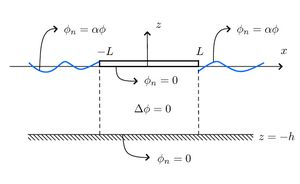
Wave scattering by a finite dock
We consider here the Frequency Domain Problem for a finite dock which occupies
the region [math]\displaystyle{ -L\lt x\lt L }[/math] (we assume [math]\displaystyle{ e^{i\omega t} }[/math] time dependence).
The water is assumed to have
constant finite depth [math]\displaystyle{ h }[/math] and the [math]\displaystyle{ z }[/math]-direction points vertically
upward with the water surface at [math]\displaystyle{ z=0 }[/math] and the sea floor at [math]\displaystyle{ z=-h }[/math]. The
boundary value problem can therefore be expressed as
[math]\displaystyle{
\Delta\phi=0, \,\, -h\lt z\lt 0,
}[/math]
[math]\displaystyle{
\phi_{z}=0, \,\, z=-h,
}[/math]
[math]\displaystyle{
\partial_z\phi=\alpha\phi, \,\, z=0,\,x \lt -L, {\rm or} \, x\gt L
}[/math]
[math]\displaystyle{
\partial_z\phi=0, \,\, z=0,\,-L\lt x\lt L,
}[/math]
We
must also apply the Sommerfeld Radiation Condition
as [math]\displaystyle{ |x|\rightarrow\infty }[/math]. This essentially implies
that the only wave at infinity is propagating away and at negative infinity there is a unit incident wave
and a wave propagating away.
We begin with the diffraction potential [math]\displaystyle{ \phi^{\mathrm{D}} }[/math] which
satisfies the following equations
[math]\displaystyle{
\Delta\phi^{\mathrm{D}} =0,\,\,-h\lt z\lt 0,
}[/math]
[math]\displaystyle{
\partial_{z}\phi^{\mathrm{D}} =0,\,\,z=-h,
}[/math]
[math]\displaystyle{
\partial_{z}\phi^{\mathrm{D}} =\alpha \phi^{\mathrm{D}},\,\,x\notin(-L,L),\,\,
z=0,
}[/math]
[math]\displaystyle{
\partial_{z}\phi^{\mathrm{D}} =0,\,\,x\in(-L,L),\,\,z=0.
}[/math]
[math]\displaystyle{ \phi^{\mathrm{D}} }[/math] satisfies the Sommerfeld Radiation Condition
[math]\displaystyle{
\frac{\partial}{\partial x} \left(\phi^{\mathrm{D}}-\phi^{\rm
I} \right) \pm k_0\left( \phi^{\mathrm{D}}-\phi^{\rm I}\right)
= 0
,\,\,\mathrm{as}
\,\,x\rightarrow\infty.
}[/math]
[math]\displaystyle{ \phi^{\mathrm{I}}\, }[/math]
is a plane wave travelling in the [math]\displaystyle{ x }[/math] direction,
[math]\displaystyle{
\phi^{\mathrm{I}}(x,z)=A \phi_0(z) e^{\mathrm{i} k x} \,
}[/math]
where [math]\displaystyle{ A }[/math] is the wave amplitude (in potential) [math]\displaystyle{ \mathrm{i} k }[/math] is
the positive imaginary solution of the Dispersion Relation for a Free Surface
(note we are assuming that the time dependence is of the form [math]\displaystyle{ \exp(-\mathrm{i}\omega t) }[/math])
and
[math]\displaystyle{
\phi_0(z) =\frac{\cosh k(z+h)}{\cosh k h}
}[/math]
As the plate is floating on the surface, we can denote it as follows:
[math]\displaystyle{
\phi^{\rm I}|_{z=0} = e^{-i kx} \,
}[/math]
Solution for Diffracted Potential
We use the Free-Surface Green Function for two-dimensional waves, with singularity at
the water surface since we are only
interested in its value at [math]\displaystyle{ z=0 }[/math]
(details about this method can be found in Integral Equation for the Finite Depth Green Function at Surface).
Using this we can transform the system of equations to
[math]\displaystyle{
\phi^{\mathrm{D}}(x) = \phi^{\mathrm{I}}(x) + \int_{-L}^{L}G(x,\xi) \alpha\phi^{\mathrm{D}}(\xi) \mathrm{d} \xi
}[/math]
Reflection and Transmission Coefficients
The Reflection and Transmission Coefficients represent the ratio of the amplitude of the reflected or transmitted wave to the amplitude of the incident wave. Conservation of energy means that [math]\displaystyle{ |R|^2+|T|^2=1\, }[/math].
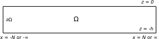
A diagram depicting the area
[math]\displaystyle{ \Omega\, }[/math] which is bounded by the rectangle
[math]\displaystyle{ \partial \Omega \, }[/math]. The rectangle
[math]\displaystyle{ \partial \Omega \, }[/math] is bounded by
[math]\displaystyle{ -h \leq z \leq 0 \, }[/math] and
[math]\displaystyle{ -\infty \leq x \leq \infty \, }[/math] or
[math]\displaystyle{ -N \leq x \leq N\, }[/math]We can calculate the Reflection and Transmission coefficients by
applying Green's theorem to [math]\displaystyle{ \phi\, }[/math] and [math]\displaystyle{ \phi^{\mathrm{I}}\, }[/math]
[math]\displaystyle{ \phi^{\mathrm{I}}\, }[/math]
is a plane wave travelling in the [math]\displaystyle{ x }[/math] direction,
[math]\displaystyle{
\phi^{\mathrm{I}}(x,z)=A \phi_0(z) e^{\mathrm{i} k x} \,
}[/math]
where [math]\displaystyle{ A }[/math] is the wave amplitude (in potential) [math]\displaystyle{ \mathrm{i} k }[/math] is
the positive imaginary solution of the Dispersion Relation for a Free Surface
(note we are assuming that the time dependence is of the form [math]\displaystyle{ \exp(-\mathrm{i}\omega t) }[/math])
and
[math]\displaystyle{
\phi_0(z) =\frac{\cosh k(z+h)}{\cosh k h}
}[/math]
We assume that [math]\displaystyle{ A=1 }[/math]. This gives us
[math]\displaystyle{
\iint_{\Omega}(\phi\Delta\phi^{\mathrm{I}} - \phi^{\mathrm{I}}\Delta\phi)\mathrm{d}x\mathrm{d}z
= \int_{\partial\Omega}(\phi \partial_n \phi^{\rm I} - \phi^{\rm I}\partial_n\phi)\mathrm{d}s = 0,
}[/math]
This means that (using the far field behaviour of the potential [math]\displaystyle{ \phi }[/math])
[math]\displaystyle{
\int_{\partial\Omega_{B}}
(\phi \partial_n \phi^{\rm I} - \phi^{\rm I}\partial_n\phi)\mathrm{d}s
+ 2k_0 R \int_{-h}^{0} \left(\phi_0(z)\right)^2 \mathrm{d}z = 0,
}[/math]
For the present case the body is present only on the surface and we therefore have
[math]\displaystyle{
\int_{-L}^{L} e^{-k_0 x} \left(\alpha \phi(x) - \partial_n \phi(x)\right)\mathrm{d}x
+ 2k_0 R \int_{-h}^{0} \left(\phi_0(z)\right)^2 \mathrm{d}z = 0
}[/math]
Therefore
[math]\displaystyle{
R = -\frac{\int_{-L}^{L} e^{-k_0 x} \left(\alpha \phi(x) - \partial_n \phi(x)\right)\mathrm{d}x }
{2 k_0 \int_{-h}^{0} \left(\phi_0(z)\right)^2 \mathrm{d}z}.
}[/math]
and using a wave incident from the right we obtain
[math]\displaystyle{
T = 1 - \frac{\int_{-L}^{L} e^{k_0 x} \left(\alpha \phi(x) - \partial_n \phi(x)\right)\mathrm{d}x }
{2 k_0 \int_{-h}^{0} \left(\phi_0(z)\right)^2 \mathrm{d}z}.
}[/math]
Note that an expression for the integral in the denominator can be found in
Eigenfunction Matching for a Semi-Infinite Dock
Matlab Code
A program to calculate the solution in elastic modes can be found here
A program to calculate the solution in elastic modes can be found here
elastic_plate_modes.m
Additional code
This program requires
Additional code
This program requires

